
- 1 Opinion: Three important types of parameters
- 1.1 Difficulty
- 1.2 Location onset and center
- 1.3 Scale
- 1.4 Which distribution is better?
- 2 Select data
- 3 Drag those sliders!
- 3.1 Gaussian (normal distribution)
- 3.2 Ex-gaussian
- 3.3 Skew normal
- 3.4 (Shifted) Log-normal
- 3.5 (Shifted) Inverse Gaussian
- 3.6 Wiener diffusion
- 3.7 Linear Ballistic Accumulator
- 3.8 Gamma
- 3.9 (Shifted) Weibull
- 4 Applied code example
- 4.1 Checking the fit
- 4.2 Understanding the parameter estimates
- 4.3 Priors and descriptives
- 5 Notes on good models for RT data
Reaction time distributions: an interactive overview
By Jonas Kristoffer Lindeløv (blog, profile).
Updated: 23 September, 2019 (source, changes).


OBS: This is the non-interactive version. Click here to go to the interactive version.
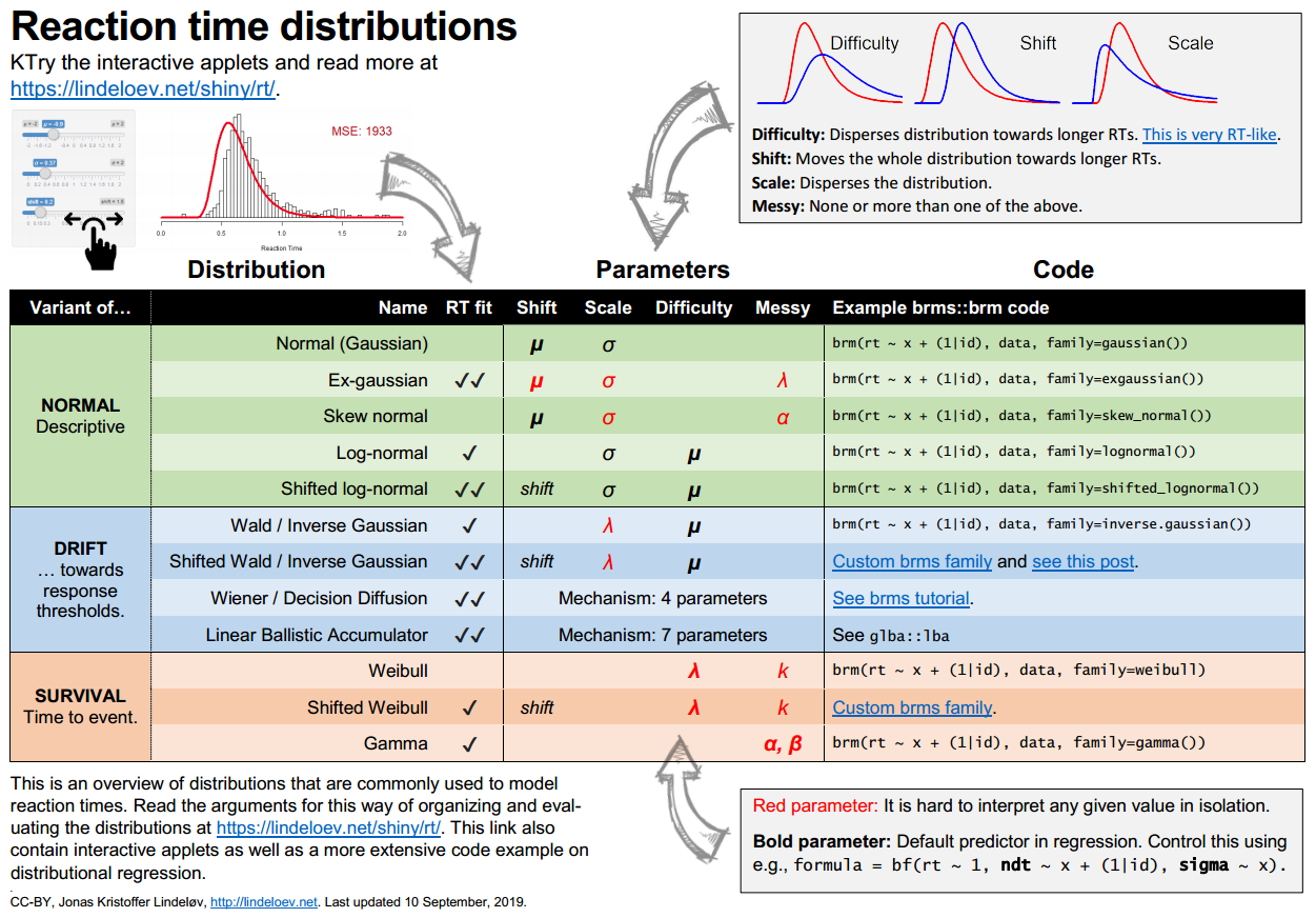
All too often, researchers use the normal distribution to model reaction times. Hopefully, this document to lower the burden of shifting to better distributions. Because the normal distribution is so poor for RTs (as you will see), the reward of shifting will be great!
The cheat sheet below gives an overview (get it in PNG or PDF). You can also skip straight to the interactive part or to the applied code example.
1 Opinion: Three important types of parameters
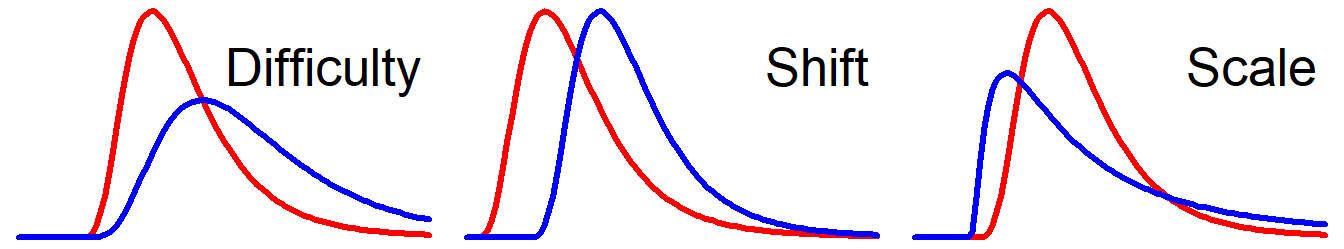
For reaction times, I’ll argue that there are three useful parameters to describe their distribution: Difficulty1, Onset2, and Scale.3 In the figure below, the blue curves show the effect of increasing each of these parameters. Try manipulating them yourself here.
1.1 Difficulty
A dominant feature of RTs is that the standard deviation increases approximately linearly with the mean (Wagenmakers et al., 2007). Reaction times are more dispersed for conditions with longer reaction times (e.g., incongruent trials) and are more condensed for conditions with shorter reaction times (e.g., congruent trials). For interpretability, it is convenient to have one parameter that changes both rather than having to regress on mean and SD separately and always interpret their interaction. Ideally, the value of the difficulty parameter should be somewhere around the center (highest density region, e.g., the median RT or the mode RT).
1.2 Location onset and center
Moves the whole distribution towards the left (longer RTs) or right (shorter RTs) without altering its shape.
- Onset: This is the earliest possible reaction time (for descriptive models where it’s often called shift) or the earliest possible start of the decision process (for mechanistic models where it’s called non-decision time). In humans, this is often around 200 ms. It’s good to have an onset-parameter since no animal can perceive or respond in 0.0 ms. Models without an onset-parameter often predict positive probabilities of impossibly short RTs.
- Center: Somewhere “in the middle” of the distribution (e.g., in the normal distribution). I argued above that we should prefer a difficulty-like parameter to model the center.
1.3 Scale
Stretches or squeezes the distribution over and above difficulty, without (severely) changing the location. This can be used to tune the distribution to population-specific or experiment-specific characteristics. For example, you would expect wider distributions in patient samples and for dual-tasks.
1.4 Which distribution is better?
It is nice when each parameter does only one thing. If they do several things at once, or if multiple parameters do the same thing, I call them messy, because you will need to tune many parameters to achieve one of the above effects. And that’s a mess for interpretability. However, if this behavior at the surface level is justified by an underlying theory that gives meaning to each parameter, I call them mechanism parameters.
With this terminology on the table, here are our three commandments:
- Bad: Distributions with messy parameters.
- Good: Distributions with an onset, a difficulty, AND a scale parameter.
- Good: Distributions with mechanism parameters.
According to these criteria, DDM, LBA, the shifted log-normal, and the inverse Gaussian are the winners on this list. If we also consider how easy it is to interpret the parameter values, I’d say that DDM and the shifted log-normal come out on top, but this is up for discussion.
2 Select data
All of the following datasets are from a single participant in a single condition.
3 Drag those sliders!
Here are some fun challenges:
One-parameter champ: For the speed/accuracy and MRT data, try (1) fitting the parameters to one dataset, (2) change the dataset, (3) see how close you can get by only changing one parameter now.
Fit champ: There is a special reward if you can fit the data so well that the mean squared error (MSE) drops below 40. Use the keyboard arrows to fine-tune parameters. The MSE in the plots is multiplied by 10.000 to give easy-to-read numbers.
Optimal champ: Use
brmsto find the optimal fits as shown in the code snippets. The empirical datasets are in thertdistspackage. Uselibrary(rtdists'),data('rr98'), anddata('speed_acc')to load them. Download the MRT data here. You can also try and use the (frequentist)gamlsspackage, though it’s harder to interpret the results.
3.1 Gaussian (normal distribution)
Models responses from a single mean with a symmetrical dispersion towards faster and slower RTs. In most cases, the normal distribution is the worst distribution to fit reaction times. For example, for typical reaction times, your fitted model will predict that more than 5% of the reaction times will be faster than the fastest RT ever recorded!
Yet, the Gaussian is by far the most frequently used analysis of reaction times because it is the default in most statistical tests, packages, and software. For example, t-tests, ANOVA, linear regression, lm, lme4::lmer, and brms::brm. Also, if your pre-processing includes computing means for each participant or condition and you use those means as data, you’ve subscribed to the Gaussian model (and thrown away a lot of wonderful data).
Parameters
- (center): the mean. It is heavily affected by the tail.
- (scale): the standard deviation. This models (symmetric) variability in RTs.
It is easy to infer these parameters from data. Here, we model by condition. is fixed across conditions. See notes on modeling and the applied example for more details.
library(brms)
fit = brm(rt ~ condition, rt_data, family=gaussian())3.2 Ex-gaussian
If you believe that responses were caused by a mix of two independent processes, (1) a Gaussian and (2) a decaying exponential, the ex-gaussian is exactly this. Most people don’t believe this but they use the ex-gaussian in a purely descriptive way because it usually has an excellent fit to RTs. See Wikipedia.
Parameters:
- (center): the mean of the gaussian. This models shorter/longer mean RTs.
- (scale): the standard deviation of the gaussian. It models symmetrical variability around .
- (messy): the decay rate of the exponential. This models the tail of long RTs. Higher –> more tail dominance over the Gaussian.
It is easy to infer these parameters from data. Here, we model by condition. and are fixed across conditions. See notes on modeling and the applied example for more details.
library(brms)
fit = brm(rt ~ condition, rt_data, family=exgaussian())3.3 Skew normal
Adds a skew to the normal (Gaussian) distribution via an extra skew-parameter. In my experience, it usually has a poorer fit to reaction times, though it is superior to the Gaussian.
Parameters:
- (center): the mean.
- (scale): the standard deviation. Changing preserves the mean but not the median. Note that when , the distribution is not symmetric, so don’t interpret it as the SD of a normal distribution.
- (messy): the skewness. When , it’s a Gaussian.
It is easy to infer these parameters from data. Here, we model by condition. and are fixed across conditions. See notes on modeling and the applied example for more details.
library(brms)
fit = brm(rt ~ condition, rt_data, family=skew_normal())3.4 (Shifted) Log-normal
When using logarithms, you model percentage increase or decrease instead of absolute differences. That is, rather than saying “RTs are 40 ms slower in incongruent trials”, your parameter(s) say that “RTs are 7% slower in incongruent trials”. This embodies the intuition that a difference of 40 ms can be huge for simple reaction times but insignificant for RTs around 10 seconds. Mathematically it is about multiplicative relationships rather than additive relationships, and this makes some sense when talking about RTs, so I’d say that the shifted log-normal is somewhere between being descriptive and mechanistic. In general, log-like models makes a lot of sense for most positive-only variables like RT.
It’s called “log-normal” because the parameters are the mean and sd of the log-transformed RTs, which is assumed to be a normal (Gaussian) distribution. For example, for simple RTs you will often see an intercept near exp(-1.5) = 0.22 seconds.
Parameters:
- (difficulty): the mean of the log-normal distribution. The mean of represents the median RT. The median RT is then .
- (scale): the standard deviation of the log-normal distribution. Increases the mean but not the median of .
- (shift): time of the earliest possible response. When , it’s a straight-up log-normal distribution with two parameters.
It is easy to infer these parameters from data. Here, we model by condition. It is log, so use exp() to back-transform. and are fixed across conditions. See notes on modeling and the applied example for more details.
library(brms)
fit = brm(rt ~ condition, rt_data, family=shifted_lognormal())3.5 (Shifted) Inverse Gaussian
… also known as the (Shifted) Wald. It is not as “inverse” of the Gaussian as it sounds. It is closely related to the Weiener / Decision Diffusion model and the LBA model in the following way (quote from Wikipedia:
The name can be misleading: it is an “inverse” only in that, while the Gaussian describes a Brownian motion’s level at a fixed time, the inverse Gaussian describes the distribution of the time a Brownian motion with positive drift takes to reach a fixed positive level.
In other words, if you have time on the x-axis and start a lot of walkers at , the Gaussian describes the distribution of their vertical location at a fixed time (t_i) while the inverse Gaussian describes the distribution of times when they cross a certain threshold on the y-axis. Like Wiener and LBA, the inverse Gaussian can be thought of as modeling a decision process, without incorporating the correctness of the response.
Parameters:
- (difficulty): The mean. Notice that this will be heavily influenced by long RTs.
- (scale): Decreases the variance but is harder to intepret since .
- (onset): time of earliest possible response. When it is a plain Inverse Gaussian or Wald distribution, i.e., only two parameters.
It is easy to infer the parameters of the (non-shifted) inverse Gaussian / Wald. Here, we model by condition. is fixed across conditions. See notes on modeling and the applied example for more details.
library(brms)
fit = brm(rt ~ condition, rt_data, family=inverse.gaussian())3.6 Wiener diffusion
Also called the Diffusion Decision Model (DDM), this is probably the most popular model focused at mechanisms. It applies to two-alternative forced-choice (2afc) scenarios and requires data on accuracy as well (scored as correct/wrong). It models RTs as a decision being made when a random walker crosses one of two thresholds (boundary). It’s clear mechanistic interpretability is a strength, but it requires some effort to understand and do. Read Ratcliff & McKoon (2008) for a motivation for the model. I like this visalization.
The diffusion idea also underlies the inverse Gaussian and the LBA model.
Parameters:
All of these are mechanism-like
- (difficulty): Boundary separation. The distance between thresholds. Longer distance –> more varied paths –> dispersed RTs.
- (onset): Non-decision time (ndt). The time at which the random walker starts.
- (difficulty): Bias. How close the walker starts to the upper threshold ( is in the middle). Higher = closer = faster and more condensed RTs.
- (difficulty): Drift Rate. The speed of the walker. Higher –> faster and more condensed RTs.
See this three-part brms tutorial by Henrik Singman on how to fit it using brms::brm and do regression on these parameters. It usually takes days or weeks to fit, but Wagenmakers (2007) made the EZ diffusion calculator which approximates the parameters in the simplest scenario. The HDDM python package can do it as well.
3.7 Linear Ballistic Accumulator
This model has some resemblance to the Wiener diffusion model in that it models latent “movements” towards decision thresholds, and is very much focused on mechanisms. It likewise applies to two-alternative forced-choice (2afc) scenarios, requiring data on accuracy as well (correct/incorrect response). Although it involves a lot of parameters, the model itself is (at least supposed to be) simpler than the diffusion model as explained in Brown & Heathcote (2008). A nice visualization from that paper escaped the paywall here.
Parameters:
All of these are mechanism-like:
- : upper bound of the starting point. The starting point is modeled as randomly drawn in this interval.
- (difficulty): response threshold (usually, ).
- (shift): the time before a “movement” is initiated, i.e., non-decision time.
- (difficulty): the mean drift rate and it’s variability (SD).
- : the mean standard deviation of the drift rate and its variability (SD)
Fit it using glba::lba(). There are some helpful distributions in the rtdists package.
3.8 Gamma
The gamma distribution is so important in statistics, that it probably spilled over to RT research as well. Although it can fit the data, it’s very hard to interpret the parameters in relation to RTs, and I will have little more to say. One could easily make a shifted Gamma, but I haven’t seen it used for the analysis of reaction times.
Parameters:
Both parameters in isolation are difficulty-like so their interaction determines scale and location. I think that this makes them messy.
- (messy): a shape parameter.
- (messy): a rate parameter.
It is easy to infer these parameters from data. Here, we model by condition. is fixed across conditions. See notes on modeling and the applied example for more details.
library(brms)
fit = brm(rt ~ condition, rt_data, family=gamma())3.9 (Shifted) Weibull
… also called the three-parameter Weibull when there is a shift parameter. For RTs, it can be understood as modeling there being an underlying rate with which underlying non-response processes are “turned into” responses over time. If , this rate is constant. If , it decreases over time. The parameter do not correspond to anything intuitive, though.
Parameters:
- (difficulty): It’s called a scale parameter for some reason, but it affects the mean, median, and mode.
- (messy): A shape parameter.
- (onset): when , it’s a straight-up Weibull distribution with the above two parameters.
It is easy to infer the parameters of the (non-shifted) Weibull from data. Here, we model by condition. It is log, so use exp() to back-transform. is fixed across conditions. See notes on modeling and the applied example for more details.
library(brms)
fit = brm(rt ~ condition, rt_data, family=weibull())4 Applied code example
We load the Wagenmakers & Brown (2007) data and pre-process it:
# Load data
library(rtdists)
data(speed_acc)

# Remove bad trials
library(tidyverse)
data = speed_acc %>%
  filter(rt > 0.18, rt < 3) %>%  # Between 180 and 3000 ms
  mutate_at(c('stim_cat', 'response'), as.character) %>%  # from factor to char
  filter(response != 'error', stim_cat == response) # Only correct responses
Now we use the shifted log-normal to ask: “Does median RT differ by condition?”. In other words, we model here, leaving the scale and the onset fixed. We include a random intercept per participant, but see my notes on formulas for RT models. In this example, it takes some time to run it because we have around 28.000 data points.
library(brms)
fit = brm(formula = rt ~ condition + (1|id),
          dat = data,
          family = shifted_lognormal(),
          file = 'fit_slog')  # Save all that hard work.
Done!
4.1 Checking the fit
Much like the interactive applets above, we can see how the parameters predict the actual data:
#plot(fit)  # Check convergence and see posteriors
pp_check(fit)  # Posterior predictive check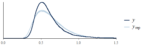
This is much better than a Gaussian. But there’s room for improvement. Mostly because is close to the earliest rt in the whole dataset, which for one participant (id #8) in one condition was 0.18 - just above the trim. The mean shortest rt was 0.28 seconds so that participant is not representative. Setting one per participant would make more sense:
formula = bf(rt ~ condition + (1|id),
             ndt ~ id)
Also, the shortest N RTs could be removed for each participant, if you can argue that they were accidental responses:
data %>%
  group_by(id) %>%
  arrange(rt) %>%
  slice(4:n())  # Remove three shortest RTs
4.2 Understanding the parameter estimates
Leaving that aside, let’s see what we learned about the parameters of the shifted log-normal model. Intercept and conditionspeed together define (the difficulty). You can see sigma (the scale) and ndt (the onset) too, so we have posteriors for all of our three parameters!
summary(fit) # See parametersPopulation-Level Effects:
Estimate Est.Error l-95% CI u-95% CI Rhat Bulk_ESS Tail_ESS
Intercept -0.69 0.04 -0.76 -0.61 1.01 508 672
conditionspeed -0.40 0.00 -0.41 -0.39 1.00 2184 2143
Family Specific Parameters:
Estimate Est.Error l-95% CI u-95% CI Rhat Bulk_ESS Tail_ESS
sigma 0.37 0.00 0.36 0.37 1.00 1839 2088
ndt 0.17 0.00 0.17 0.18 1.00 1576 1724Because and define the log-normal distribution, they are on a log scale. This means that we expect a median RT of seconds for condition “accuracy” (the intercept), and a median RT of exp(-0.69 -0.40) = 0.34 seconds for condition “speed”. If you get confused about these transformations, worry not. brms has you covered, no matter the distribution:
marginal_effects(fit)  # Back-transformed parameter estimates
marginal_effects(fit, method='predict')  # Same, but for responses
We are very certain that they respond faster for “speed” because the upper bound of the credible interval is much smaller than zero. We could test this more directly:
hypothesis(fit, 'conditionspeed < 0') # Numerically4.3 Priors and descriptives
I cut corners here for the sake of brevity. Instead of going with the default priors, I would have specified something sensible and run brm(..., prior=prior). Mostly as regularization. There is so much data that most priors will be overwhelmed.
# See which priors you can set for this model
get_prior(rt ~ condition + (1|id), speed_acc, family = shifted_lognormal())

# Define them
prior = c(
  set_prior('normal(-1, 0.5)', class = 'Intercept'),  # around exp(-1) = 0.36 secs
  set_prior('normal(0.4, 0.3)', class = 'sigma'),  # SD of individual rts in log-units
  set_prior('normal(0, 0.3)', class = 'b'),  # around exp(-1) - exp(-1 + 0.3) = 150 ms effect in either direction
  set_prior('normal(0.3, 0.1)', class = 'sd')  # some variability between participants
)
I would probably also have checked that the pre-processing worked by plotting the response distributions of a few participants:
data_plot = filter(data, id %in% c(1, 8, 15))

ggplot(data_plot, aes(x=rt)) +
    geom_histogram(aes(fill=condition), alpha=0.5, bins=60) +
    facet_grid(~id) +  # One panel per id
    coord_cartesian(xlim=c(0, 1.6))  # Zoom in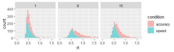
5 Notes on good models for RT data
Throughout this document, I have used a simple model: rt ~ condition to demo code. For real-world data, you probably know a lot more about the data generating process. This is a better typical recipe:
rt ~ condition + covariates + (condition | id) + (1|nuisance)This could be an example of using this recipe:
rt ~ congruent + trial_no + bad_lag1 + (congruent|id) + (1|counterbalancing)Let’s unpack this:
conditionis our contrast of interest. This can be a variable coded as congruent/incongruent, the number of items in a visual search, or something else. It can also be an interaction. I just did an analysis where I had acongruent:conditionterm to model a congruency effect per condition.covariatescould be, e.g.,trial_no + bad_lag1, i.e., the effect of time (people typically get faster with practice) and longer RTs on the first trial in a block (you need to code this variable). It is often a good idea to these to help the model fit, and to them (possible for continuous and binary predictors) so that the effect ofconditionrepresents the mean of the other conditions rather than a certain combination. You can usescaleto scale and center.(condition | id)models the expected individual differences in generalrt, and allows the effect ofconditionto vary between participants. The practical effect of specifying a random effect rather than a fixedcondition:ideffect is that you get shrinkage in the former, naturally imposing a bit of control for outliers. Unfortunately, complicated random effects sometimes increase computation time considerably.(1 | nuisance)is a way to let the model “understand” a structure in the data, without having it affect the fixed parameter estimates. If you have a factorial design, the otherwise non-modeled design variables would generally go here.
“Difficulty” is a term borrowed from Wagenmakers & Brown (2007), but it is not standard↩
Some distributions are parameterized using rate which is the inverse of location center.↩
Many distributions include a shape parameter, but since all RT distributions have approximately the same shape, I’d rather pick a distribution which inherently has the “right” shape, than model this using a parameter.↩