Mann-Whitney is (almost) an independent-sample t-test on ranks
Jonas Kristoffer Lindeløv
This document presents the close relationship between the p-values of the Mann-Whitney U test and a two-sample t-test on the ranked data. It is an appendix to the post “Common statistical tests as linear models”.
TL;DR: I argue below that starting at N = 12, 5the t-test is a reasonable approximation. For N > 30, it is almost exact.
Since the Mann-Whitney U is a Wilcoxon test, it may also be worth looking at my equivalent simulation about whether Wilcoxon Signed Rank test is one-sample t-test on ranks (hint: almost yes).
1 Small example
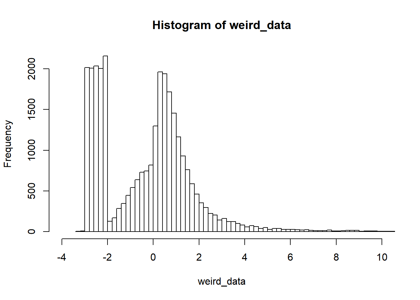
First, let’s find a way tocreate some clearly non-normal data. How about this ex-gaussian + uniform values in the negative end:
weird_data = c(rnorm(10000), exp(rnorm(10000)), runif(10000, min=-3, max=-2))
hist(weird_data, breaks=200, xlim=c(-4, 10))
… and then compute p-values using Wilcoxon and “ranked t-test” respectively:
# Test differences between these two datasets
x = sample(weird_data, 50)
y = rnorm(50)

# Wilcoxon / Mann-Whitney U
wilcox = wilcox.test(x, y)

# Parametric on ranks
ranks = rank(c(x, y))  # Look up for data
ranked_x = ranks[1:length(x)]  # Select one
ranked_y = ranks[-(1:length(x))]  # Select the other
ttest = t.test(ranked_x, ranked_y)  # Comparable to Wilcoxon?

# You can also do it as a linear model
summary(lm(ranks ~ I(rep(c('x', 'y'), each=50))))
##
## Call:
## lm(formula = ranks ~ I(rep(c("x", "y"), each = 50)))
##
## Residuals:
## Min 1Q Median 3Q Max
## -49.98 -24.27 -0.48 24.51 49.02
##
## Coefficients:
## Estimate Std. Error t value Pr(>|t|)
## (Intercept) 50.980 4.123 12.364 <2e-16 ***
## I(rep(c("x", "y"), each = 50))y -0.960 5.831 -0.165 0.87
## ---
## Signif. codes: 0 '***' 0.001 '**' 0.01 '*' 0.05 '.' 0.1 ' ' 1
##
## Residual standard error: 29.16 on 98 degrees of freedom
## Multiple R-squared: 0.0002765, Adjusted R-squared: -0.009925
## F-statistic: 0.02711 on 1 and 98 DF, p-value: 0.8696# Compare p-values
rbind(wilcoxon = wilcox$p.value,
ttest = ttest$p.value)## [,1]
## wilcoxon 0.8713021
## ttest 0.8695861Pretty close! But does it hold up to more scrutiny? Let’s find out…
2 Simulation
Let’s do what we did above, but running a few thousand simulations for different N and means (mu):
library(tidyverse)

# Parameters
Ns = c(seq(from=6, to=20, by=2), 30, 50, 80)
mus = c(0, 0.5, 1)  # Means
PERMUTATIONS = 1:200

# Run it
D = expand.grid(set=PERMUTATIONS, mu=mus, N=Ns) %>%
  mutate(
    # Generate data. One normal and one weird
    data = map2(N, mu, ~cbind(sample(weird_data, .x), .y + rnorm(.x))),

    # Built-in
    mann_raw = map(data, ~ wilcox.test(.x[,1], .x[,2])),

    # Ttest
    ranked_value = map(data, ~ rank(c(.x))),  # As 1D ranked vector for t.test
    ttest_raw = map2(ranked_value, N, ~t.test(.x[1:.y], .x[-(1:.y)], var.equal=TRUE)),

    # Tidy it up
    mann = map(mann_raw, broom::tidy),
    ttest = map(ttest_raw, broom::tidy)
  ) %>%

  # Get as columns instead of lists; then remove "old" columns
  unnest(mann, ttest, .sep='_') %>%
  select(-data, -mann_raw, -ranked_value, -ttest_raw)

head(D)
2.1 Inspect p-values
Let’s take a look at how the p-values from the “ranked t-test” compare to Mann-Whitney p-values:
D$N = factor(D$N)  # Make N a factor for prettier plotting

library(ggplot2)
library(patchwork)

# A straight-up comparison of the p-values
p_relative = ggplot(D, aes(x=mann_p.value, y=ttest_p.value, color=N)) +
  geom_line() +
  geom_vline(xintercept=0.05, lty=2) +
  geom_hline(yintercept=0.05, lty=2) +

  labs(title='Absolute relation', x = 'Mann-Whitney p-value', y = 'T-test p-value') +
  #coord_cartesian(xlim=c(0, 0.10), ylim=c(0, 0.11)) +
  theme_gray(13) +
  guides(color=FALSE)

# Looking at the difference (error) between p-values
p_error_all = ggplot(D, aes(x=mann_p.value, y=ttest_p.value-mann_p.value, color=N)) +
  geom_line() +
  geom_vline(xintercept=0.05, lty=2) +

  labs(title='Error', x = 'Mann-Whitney p-value', y = 'T-test p-value deviation') +
  theme_gray(13) +
  guides(color=FALSE)

# Same, but zoomed in around p=0.05
p_error_zoom = ggplot(D, aes(x=mann_p.value, y=ttest_p.value-mann_p.value, color=N)) +
  geom_line() +
  geom_vline(xintercept=0.05, lty=2) +

  labs(title='Zoomed error', x = 'Mann-Whitney p-value', y = 'T-test p-value deviation') +
  coord_cartesian(xlim=c(0, 0.10), ylim=c(-0.020, 0.000)) +
  theme_gray(13)

# Show it. Patchwork is your friend!
p_relative + p_error_all + p_error_zoom
3 Conclusion
I would say that the paired t-test on ranked data is a reasonable approximation starting at N = 12 which is where p is off by less than 0.5% in the “critical” region around p=5%. It is virtually perfect when N > 30.
This holds regardless of the normality of the data and the magnitude of the difference between the samples. I have not presented this in more detail here for the sake of brevity.