
Poisson and negative-binomial change point analysis
2026-10-26
Source:vignettes/poisson.Rmd
poisson.RmdThe Poisson and negative-binomial distributions model counts observed
within comparable units of time, space, or exposure. The worked example
below uses Poisson regression; a later section explains the additional
shape parameter and priors in
negbinomial().
Coal mining disasters
A dataset on coal mining disasters has grown very popular in the
change point literature (available in boot::coal). It
contains a timestamp of each coal mining disaster from 1851 to 1962. By
counting the number of events within each year (fixed time frame), we
have something very Poisson-friendly. Note that years without disasters
must be included as zeros:
# Number of disasters by year, including years with zero disasters (no data rows)
year = factor(floor(boot::coal$date), levels = 1851:1962)
df = data.frame(date = 1851:1962, n = as.vector(table(year)))

# See it
head(df)
## date n
## 1 1851 4
## 2 1852 5
## 3 1853 4
## 4 1854 1
## 5 1855 0
## 6 1856 4The number of events (n) as a function of year
(date) is typically modeled as a change between two
intercepts. This is very simple to do in mcp:
library(mcp)
future::plan(future::multisession, workers = 3)
model = list(
  n ~ 1,  # intercept-only
  ~ 1  # intercept-only
)

fit = mcp(model, data = df, family = poisson(), par_x = "date")
Let us see the two intercepts (lambda in log-units) and the change point (in years):
result = summary(fit)
result
## Family: poisson
## Links: mu = log
## Draws: 9000 (3 chains with iter = 3000)
## Segments:
## 1: n ~ 1
## 2: ~ 1
##
## Change point parameters:
## parameter mean sd lower upper rhat ess_bulk ess_tail
## cp_1 1890.5 2.5 1886.1 1896.5 1.00 1944 990
##
## Population-level parameters:
## parameter mean sd lower upper rhat ess_bulk ess_tail
## Intercept_1 1.131 0.094 0.944 1.313 1.00 4302 4741
## Intercept_2 -0.09 0.13 -0.35 0.15 1.00 4472 5006We can see that the model ran well with good convergence and large effective sample sizes. At a first glance, the change point is estimated to lie between the years 1886 and 1897 (95% interval).
Let us take a more direct look, using the default mcp
plot:
plot(fit)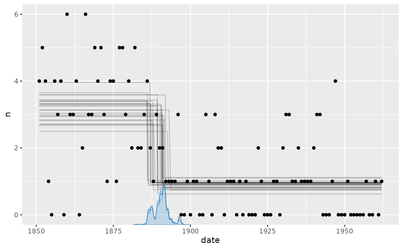
It seems to fit the data well, but we can see that the change point probability “lumps” around particular data points. Years with a very low number of disasters abruptly increase the probability that the change to a lower disaster rate has taken place. The posterior distributions of change points regularly take these “weird” forms, i.e., not well-described by our toolbox of parameterized distributions.
We can see this more clearly if plotting the posteriors. We include a traceplot too, just to check convergence visually.
plot_pars(fit)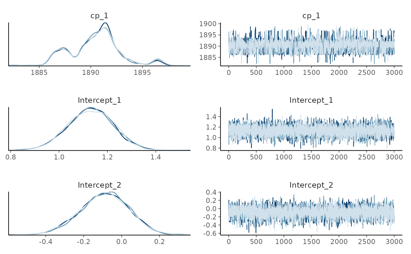
Priors for Poisson models
Brief overview of all default priors
poisson() defaults to link = 'log', meaning
that we have to exponentiate the estimates to get the “raw” Poisson
parameter \lambda. \lambda has the nice property of being the
mean number of events. So the rate is around 3.1 disasters per year in
segment 1 and 0.91 in segment 2. Exponentiating the posterior mean of
the log-rate gives approximately the posterior median of \lambda, not its mean. For the posterior
mean, exponentiate the draws before averaging, e.g.,
mean(exp(as_draws_df(fit)$Intercept_1)), or use
fitted(fit).
The intercept prior is a normal distribution centered on the median
of log(n), with zeros replaced by 0.1 (as in
brms), and scale equal to the maximum of 2.5 and its MAD.
Replacing zeros keeps the log finite and the minimum scale avoids an
accidentally narrow prior.
Coefficients are autoscaled
as in rstanarm, e.g.,
dnorm(0, 2.5 / sd(column)), and group-level SDs default to
half-normal priors. These normal priors avoid the infinite expected
counts that heavier Student-t tails imply under the log link (read more).
prior_summary(fit)## # A tibble: 3 × 5
## parameter segment dpar prior bounds
## <chr> <int> <chr> <chr> <chr>
## 1 cp_1 2 NA dunif(1851, 1962) [1851, 1962], ordered
## 2 Intercept_1 1 mu dnorm(0, 2.5) none
## 3 Intercept_2 2 mu dnorm(0, 2.5) noneThe default prior on the change point restricts it to the observed range. The coefficient priors are deliberately broad defaults, so update them with more informed priors for your particular case when possible, e.g.:
Negative-binomial extension
negbinomial() uses log links for its conditional mean
mu and, when modeled, its overdispersion
shape, where \operatorname{Var}(y) = \mu + \mu^2 /
\mathit{shape}. Its mean priors are the same as for
poisson().
When no shape() formula is supplied,
shape_1 is the shape itself (like sigma_1 in
gaussian()) with an inverse-gamma(0.4, 0.3) prior, matching
brms. It covers both strong overdispersion and the
large-shape Poisson limit.
An explicit shape() formula models log-shape.
Harmonizing with log-mean coefficients, its intercept and contrasts
default to dnorm(0, 2.5) and slopes to
dnorm(0, 2.5 / sd(column)) (group SDs default to
dnorm(0, ...) T(0, )). Where brms uses flat
coefficients and a Student-t intercept, mcp uses proper
normal priors to avoid heavy tails that pull shape toward extreme
overdispersion. Shape regression can be weakly identified, so informed
priors may be useful.
Modeling rates using offset()
When modeling event counts where exposure (e.g., person-years, area,
or population size) varies across observations, you can model rates
\lambda = \text{Count} /
\text{exposure} on the log link by supplying
offset(log(exposure)):
# Example: Event counts over varying observation durations (as here) or population
model = list(
  events ~ 1 + year + offset(log(exposure)),  # Segment 1
  ~ 1 + year + offset(log(exposure))          # Segment 2
)

fit = mcp(model, data = df, family = poisson())  # implicit link = "log"
fitted() returns expected counts given each row’s
exposure. To get expected rates per unit of exposure, set the exposure
to 1 in newdata, so that the offset is \log(1) = 0:
This works the same way for predict(), which then
returns predicted counts at unit exposure. The
fitted(..., rate = TRUE) argument does not apply to Poisson
or negative-binomial models; it is only for binomial models, where it
converts counts to proportions of trials.
Adding a categorical predictor to the model, you can also model rate
ratios. When an offset is present, mcp automatically shifts
the default intercept prior from centering on observed log-counts to
observed log-rates (\log(y) -
\text{offset}), keeping the minimum scale at 2.5.
Note on
par_xvs. cumulative exposure:
The offset is evaluated per row as local exposure for that observation. Ifpar_xrepresents continuous cumulative time from an origin (e.g., [0, t_i]), usingoffset(log(par_x))does not integrate piecewise rates across prior segments; instead, the current segment’s rate is applied to the total duration. If your data consists of discrete time intervals (bins) of duration \Delta t_i, usingoffset(log(delta_t))is valid.
Model comparison
Despite the popularity of this dataset, a question rarely asked is what the evidence is that there is a change point at all. Let us fit two models without change points and use approximate leave-one-out cross-validation to see how the predictive performance of the two models compare.
A flat model and a one-decay model. The intercept in mcp
is at date = 0, far from the data, so we measure the decay
from the first year (I(date - 1851)) to reduce the
posterior correlation between intercept and slope. This helps
sampling:
# Fit an intercept-only model
fit_flat = mcp(list(n ~ 1), data = df, family=poisson(), par_x = "date")
fit_decay = mcp(list(n ~ 1 + I(date - 1851)), data = df, family = poisson(), par_x = "date")


plot(fit_flat) + plot(fit_decay)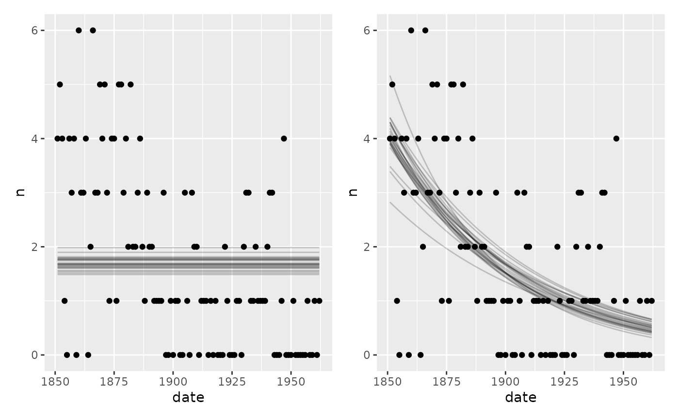
Now we compute and compare the LOO ELPDs:
fit_loo = loo(fit)## Warning: Some Pareto k diagnostic values are too high. See help('pareto-k-diagnostic') for details.
loo::loo_compare(fit_loo, fit_flat_loo, fit_decay_loo)## model elpd_diff se_diff p_worse diag_diff diag_elpd
## model1 0.0 0.0 NA 4 k_psis > 0.7
## model3 -3.2 3.6 0.82 |elpd_diff| < 4
## model2 -32.9 8.3 1.00##
## Diagnostic flags present.
## See ?`loo-glossary` (sections `diag_diff` and `diag_elpd`)
## or https://mc-stan.org/loo/reference/loo-glossary.html.The flat model is clearly worse, with
elpd_diff / se_diff around 4, so the disaster rate did
decrease. The change point model is preferred over the decay model, but
the difference is smaller than its standard error. The
diag_elpd column also flags a few observations with high
Pareto k values in the change point
model, so its PSIS-LOO estimate is less reliable. Taken together, the
data cannot clearly distinguish an abrupt change from a gradual decay.
Another approach is to look at the model weights:
loo_list = list(fit_loo, fit_flat_loo, fit_decay_loo)
loo::loo_model_weights(loo_list, method="pseudobma")
## Method: pseudo-BMA+ with Bayesian bootstrap
## ------
## weight
## model1 0.794
## model2 0.000
## model3 0.206Again, the change point model is preferred and the weights show the
same ranking as implied by loo_compare, but the decay model
retains a non-negligible weight.
JAGS code for the Poisson example
Here is the JAGS code for the full Poisson change-point model above.
fit$jags_code## model {
## # Change points
## cp_0 = min(date)
## cp_1 ~ dunif(cp_0, cp_2) # Uniform within the observed range of date
## cp_2 = max(date)
##
## # Priors for population-level effects
## Intercept_1 ~ dnorm(0, 1/(2.5)^2) # Robustly centered log-count intercept with a minimum scale of 2.5
## Intercept_2 ~ dnorm(0, 1/(2.5)^2) # Robustly centered log-count intercept with a minimum scale of 2.5
##
## # Model and likelihood
## for (i_ in 1:length(date)) {
## # date measured from each segment's change point
## x_local_1_[i_] = min(date[i_], cp_1)
## x_local_2_[i_] = min(date[i_], cp_2) - cp_1
##
## # Formula for mu
## link_mu_[i_] =
## (date[i_] >= cp_0) * (date[i_] < cp_1) * inprod(rhs_matrix_[i_, c(1)], c(Intercept_1)) * 1 +
## (date[i_] >= cp_1) * inprod(rhs_matrix_[i_, c(2)], c(Intercept_2)) * 1
##
## # Likelihood for family = poisson()
## mu_[i_] = exp(link_mu_[i_])
## n[i_] ~ dpois(mu_[i_])
## }
## }