
Given a model (a list of segment formulas), mcp infers the posterior
distributions of the parameters of each segment as well as the change points
between segments. See details or the mcp website.
Usage
mcp(
  model,
  data,
  prior = list(),
  family = gaussian(),
  par_x = NULL,
  sample = "post",
  chains = 3,
  iter = 3000,
  warmup = 1000,
  inits = NULL,
  jags_code = NULL,
  seed = NULL,
  diagnostics = list(),
  quiet = getOption("mcp_quiet", FALSE),
  cores = lifecycle::deprecated(),
  adapt = lifecycle::deprecated()
)
Arguments
- model
A list of formulas, one for each segment, in the format
model = list(response ~ predictors, ~ cp(...) + predictors), wherecp()is optional. See mcp-formula for how segments connect and the full formula syntax. Read more.- data
Table-like data in long format (data.frame, tibble, data.table, etc.) with syntactic column names. The response variable can contain missing values, which will be imputed jointly with the parameters. Read more.
- prior
Named list, e.g.,
prior = list(cp_1 = "dunif(0, 100)", Intercept_1 = "dnorm(0, 1)"). List names are parameter names (cp_1,Intercept_1,x_2,sigma_1, etc.) and values are a distribution string (e.g.,"dnorm(0, 1) T(0, )"), a constant (e.g.,-2.1), or the name of another parameter to share its value. OBS: Distributions use JAGS names but SD/scale instead of JAGS precision, sodnorm(0, 0.001)is a very narrow prior. Weakly informative defaults are used where priors are not specified; see them withprior_summary(). See mcp-priors for the full syntax. Read more.- family
A supported family and link function:
gaussian(link = "identity")orgaussian(link = "log")binomial()orbernoulli()withlink = "logit","probit", or"identity"poisson(link = "log")orpoisson(link = "identity")negbinomial(link = "log", link_shape = "log")
- par_x
String. Name of the change-point variable, i.e., the data column on which change points are located.
NULL(default) auto-detects it as the only continuous variable in the formulas.- sample
One of
"post": Sample the posterior."prior": Sample only the prior. Useprior = TRUEexplicitly in plots, summaries, and other methods to select prior draws."both": Sample both prior and posterior. Plots, summaries, etc. will default to using the posterior. Useprior = TRUEto select prior draws."none"orFALSE: Do not sample. Returns an mcpfit object without draws (an "empty fit"). This is useful if you only want to check prior strings (fit$prior), the JAGS model (fit$jags_code), etc.
- chains
Positive integer. Number of chains to run.
- iter
Positive integer. Number of post-warmup draws from each chain. The total number of draws is
iter * chains.- warmup
Positive integer. Number of initial iterations per chain which are discarded before sampling. Set higher if needed for sampler adaptation; use diagnostics to assess convergence.
- inits
A named list of initial values for the parameters, e.g.,
list(Intercept_1 = 10), or a list of such lists with one per chain. This can be useful if a model fails to converge (read more). Names must be parameters inmcp_pars(). Parameters with constant priors and parameters that are reparameterized for faster sampling cannot be initialized (seemcp_reparamin mcp-package). Initial values for change points must be ordered. Defaults toNULLwhere all chains start at equally spaced change points and the prior medians. User-providedinitstake precedence.- jags_code
String. JAGS code to sample instead of the code that
mcpwrites. This is an expert option for edits tofit$jags_codethat keep the parameters inmcp_pars(), the data, and the likelihood. Only the parameters inmcp_pars()are monitored. R-side simulation and prediction methods continue to use themcpformulas (with warning), sofitted(),predict(),plot(),loo(), etc. are wrong if the custom code changes the formula or likelihood. The written JAGS code is not a stable interface and may change betweenmcpversions.jags_codeis planned for deprecation once a future mcp release brings custom families and tooling to runfit$jags_codedirectly in JAGS. Read more about howmcpwrites JAGS code.- seed
NULLor a positive integer. Seed for the JAGS random-number generators. IfNULL(default), the seed is drawn from R's random-number generator, soset.seed()beforemcp()also makes sampling reproducible.- diagnostics
Named list of diagnostic warning thresholds. Available elements are
rhat = 1.01,ess_bulk = 400,ess_tail = 400,ar = 0.10, andma = 0.10. An empty list uses these defaults; a partial list overrides only the supplied values. Set an element toNULLto disable that diagnostic, or useFALSEto disable all configurable diagnostic warnings. Insummary.mcpfit(),NULLinherits the settings used to fit the model, while a list orFALSEoverrides the diagnostic footer.- quiet
Logical. Suppress routine JAGS output and mcp sampling-status messages? Defaults to
FALSE. Useoptions(mcp_quiet = TRUE)to change the default for the session.- cores
Deprecated and ignored. Configure parallel processing with a future plan instead, for example
future::plan(future::multisession, workers = 3). With the default future plan, chains are sampled sequentially. The argument remains available for backwards compatibility.- adapt
Deprecated; use
warmupinstead.
Value
An mcpfit object.
Details
Here is the demo model, which ships already fitted as demo_fit (see also mcp_example("demo")):
model = list(
  response ~ 1,  # Plateau in the first segment (Intercept_1)
  ~ 0 + time,    # Joined slope (time_2) in segment 2 which starts at cp_1
  ~ 1 + time     # Disjoined slope (Intercept_3, time_3) at cp_2
)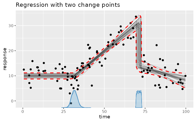
Segment 2 continues from where the plateau left off, while segment 3 starts afresh with a new intercept. See mcp-formula for the rules of how segments connect, the full formula syntax, and the underlying model. See mcp-priors for how to specify priors. See the mcp website for worked examples of all model features.
References
Lindeløv, J. K. (2020). mcp: An R Package for Regression With Multiple Change Points. OSF Preprints. doi:10.31219/osf.io/fzqxv Introduces the
mcppackage, formula syntax, default priors, and workflow for regression with multiple change points across generalized linear and time-series models. Newer-than-2020 versions of the paper may be available at that link. Please cite the newest version.Carlin, B. P., Gelfand, A. E., & Smith, A. F. (1992). Hierarchical Bayesian Analysis of Changepoint Problems. Applied Statistics, 41(2), 389–405. doi:10.2307/2347570 Introduced Gibbs sampling for hierarchical Bayesian change-point models, the computational approach that BUGS and JAGS build on.
Author
Jonas Kristoffer Lindeløv jonas@lindeloev.dk
Examples
# \donttest{
# Define the segments using formulas. A change point is estimated between each formula.
model = list(
response ~ 1, # Plateau in the first segment (Intercept_1)
~ 0 + time, # Joined slope (time_2) in segment 2 which starts at cp_1
~ 1 + time # Disjoined slope (Intercept_3, time_3) at cp_2
)
# Fit it and sample the prior too.
# future::plan(future::multisession, workers = 3) # Uncomment for parallel sampling
data = mcp_example_data("demo") # Simulated data example
demo_fit = mcp(model, data = data, sample = "both", seed = 42)
# See parameter estimates
summary(demo_fit)
#> Family: gaussian
#> Links: mu = identity; sigma = identity
#> Draws: 9000 (3 chains with iter = 3000)
#> Segments:
#> 1: response ~ 1
#> 2: ~ 0 + time
#> 3: ~ 1 + time
#>
#> Change point parameters:
#> parameter mean sd lower upper rhat ess_bulk ess_tail sim match
#> cp_1 31.8 1.7 28.5 35.1 1.00 3249 4358 30.0 OK
#> cp_2 71.1 1.0 69.5 72.8 1.00 3660 6245 70.0 OK
#>
#> Population-level parameters:
#> parameter mean sd lower upper rhat ess_bulk ess_tail sim match
#> Intercept_1 9.96 0.65 8.69 11.25 1.00 4919 6791 10.00 OK
#> time_2 0.547 0.048 0.456 0.643 1.00 5176 6667 0.500 OK
#> Intercept_3 13.9 1.4 11.3 16.7 1.00 2254 4267 15.0 OK
#> time_3 -0.205 0.084 -0.372 -0.039 1.00 1238 2159 -0.300 OK
#> sigma_1 3.87 0.29 3.35 4.47 1.00 5025 5407 3.50 OK
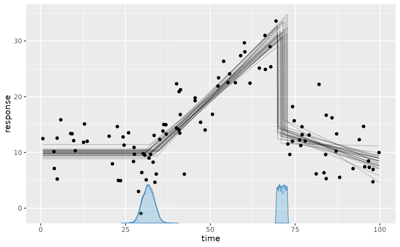
# Visual inspection of the results
plot(demo_fit) # Visualization of model fit/predictions
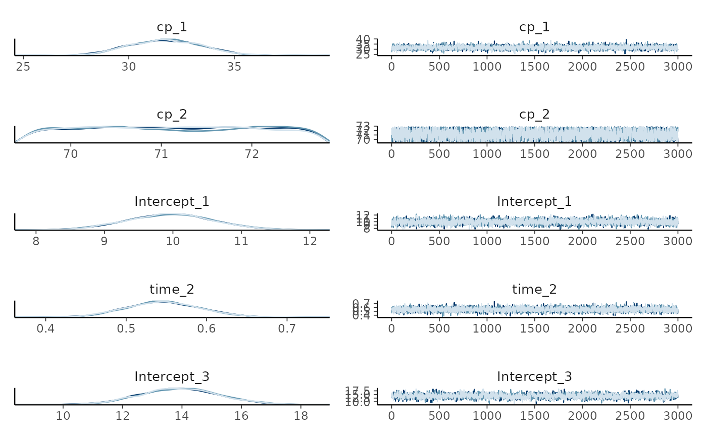
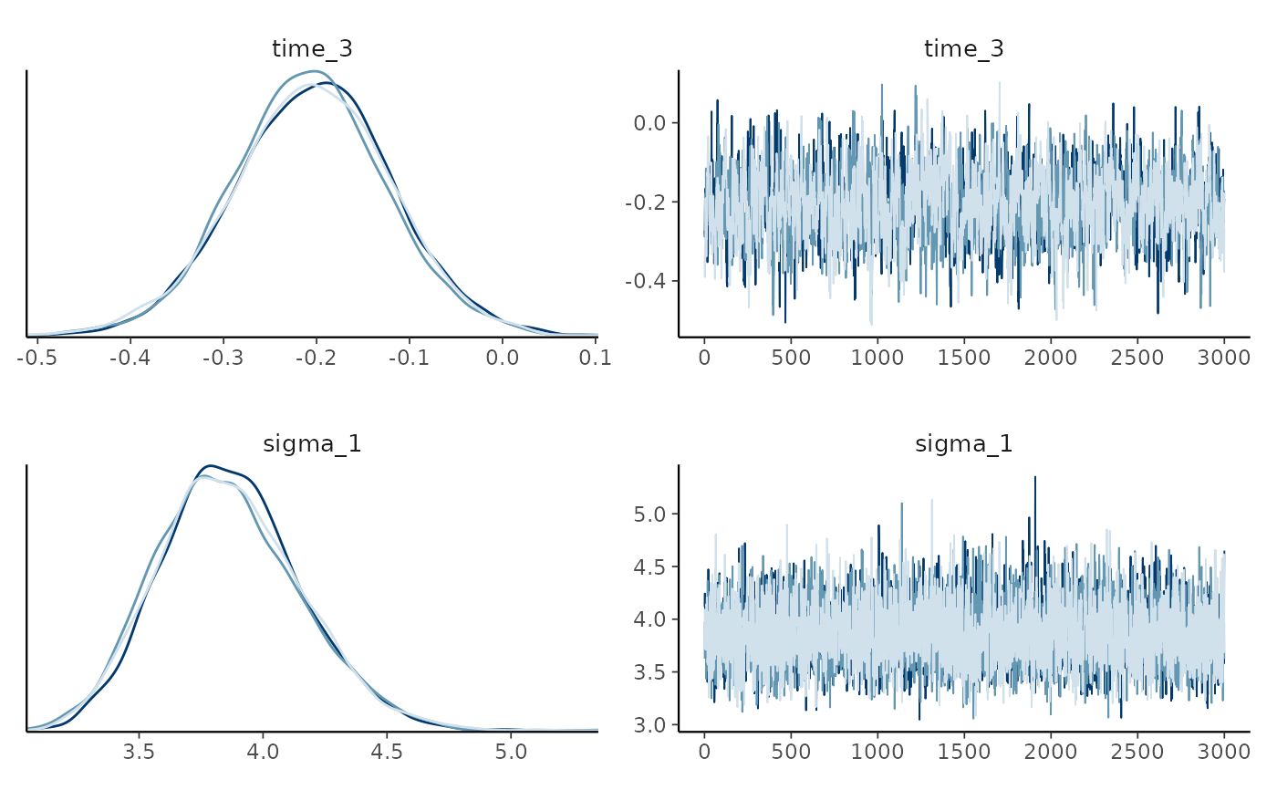
 plot_pars(demo_fit) # Parameter distributions
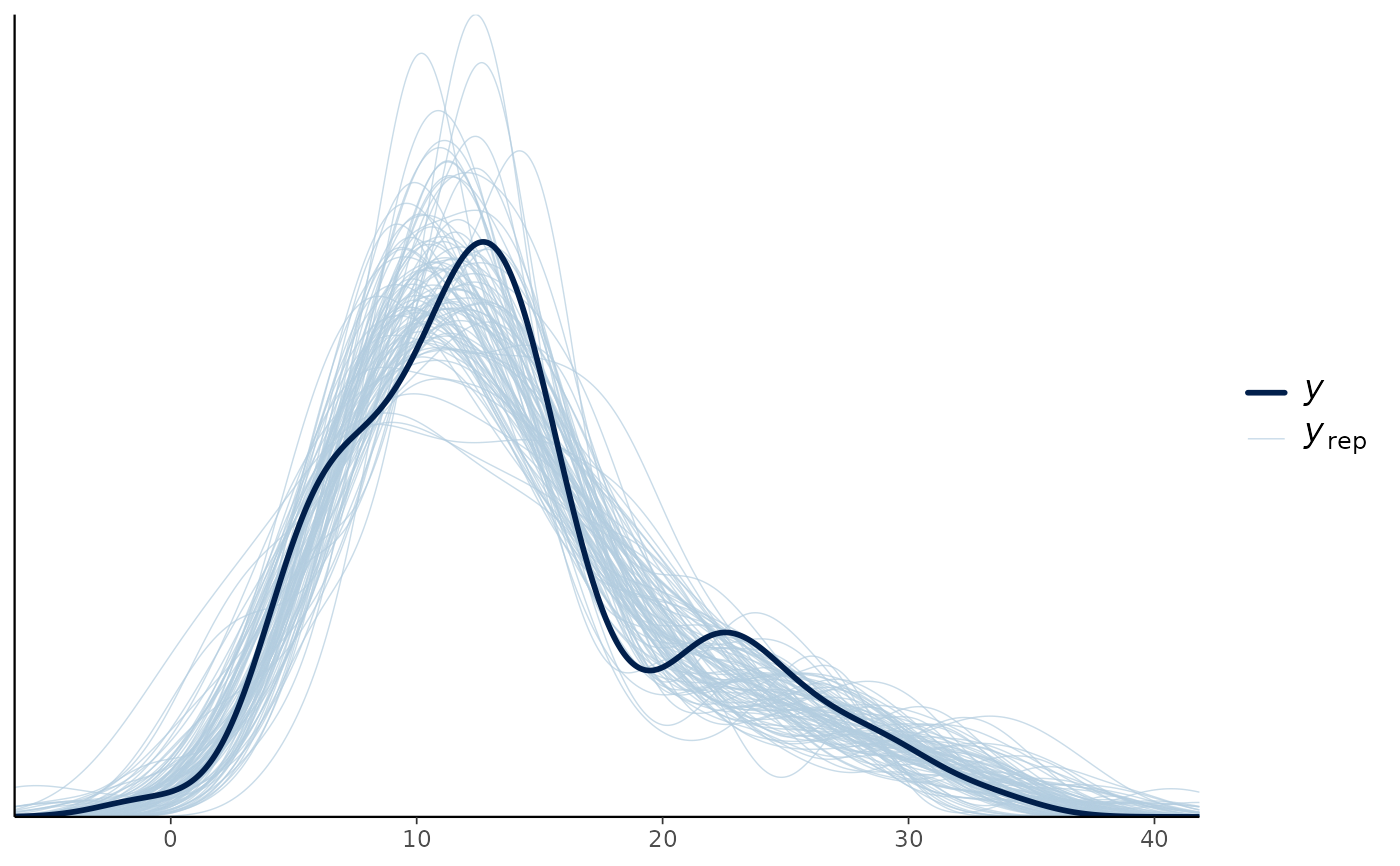
 pp_check(demo_fit) # Prior/Posterior predictive checks
 # Test a hypothesis
hypothesis(demo_fit, "cp_1 > 30")
#> # A tibble: 1 × 7
#> hypothesis mean sd lower upper prob BF
#> <chr> <dbl> <dbl> <dbl> <dbl> <dbl> <dbl>
#> 1 cp_1 - 30 > 0 1.75 1.74 -1.52 5.08 0.836 5.13
# Make predictions
head(fitted(demo_fit))
#> # A tibble: 6 × 6
#> response time .mean .sd .lower .upper
#> <dbl> <dbl> <dbl> <dbl> <dbl> <dbl>
#> 1 12.2 76.3 12.9 1.01 10.9 14.9
#> 2 6.35 83.5 11.4 0.714 10.0 12.8
#> 3 28.0 60.2 25.5 0.897 23.7 27.2
#> 4 15.7 74.7 13.2 1.11 11.1 15.4
#> 5 16.2 85.9 10.9 0.708 9.54 12.3
#> 6 22.3 40.1 14.5 0.649 13.1 15.6
head(predict(demo_fit))
#> # A tibble: 6 × 6
#> response time .mean .sd .lower .upper
#> <dbl> <dbl> <dbl> <dbl> <dbl> <dbl>
#> 1 12.2 76.3 12.9 4.01 5.01 20.8
#> 2 6.35 83.5 11.4 3.94 3.67 19.2
#> 3 28.0 60.2 25.5 3.98 17.6 33.3
#> 4 15.7 74.7 13.2 4.03 5.29 21.1
#> 5 16.2 85.9 10.9 3.94 3.18 18.7
#> 6 22.3 40.1 14.5 3.93 6.73 22.2
head(predict(demo_fit, newdata = data.frame(time = c(55.545, 80, 132))))
#> # A tibble: 3 × 5
#> time .mean .sd .lower .upper
#> <dbl> <dbl> <dbl> <dbl> <dbl>
#> 1 55.5 22.9 3.95 15.2 30.7
#> 2 80 12.1 3.96 4.35 19.9
#> 3 132 1.48 5.58 -9.52 12.4
# Compare to a one-intercept-only model (no change points) with default prior
model_null = list(response ~ 1)
fit_null = mcp(model_null, data = data, par_x = "time") # fit another model here
demo_loo = loo(demo_fit)
null_loo = loo(fit_null)
loo_compare(demo_loo, null_loo)
#> model elpd_diff se_diff p_worse diag_diff diag_elpd
#> model1 0.0 0.0 NA
#> model2 -58.1 9.1 1.00
# Inspect the prior. Useful for prior predictive checks.
summary(demo_fit, prior = TRUE)
#> Family: gaussian
#> Links: mu = identity; sigma = identity
#> Draws: 9000 (3 chains with iter = 3000)
#> Segments:
#> 1: response ~ 1
#> 2: ~ 0 + time
#> 3: ~ 1 + time
#>
#> Change point parameters:
#> parameter mean sd lower upper rhat ess_bulk ess_tail sim match
#> cp_1 34 23 2 84 1.00 3984 5301 30 OK
#> cp_2 67 23 17 98 1.00 3496 5260 70 OK
#>
#> Population-level parameters:
#> parameter mean sd lower upper rhat ess_bulk ess_tail sim match
#> Intercept_1 14 18 -20 48 1.00 9356 8910 10 OK
#> time_2 -0.01 0.63 -1.24 1.22 1.00 9087 8988 0.50 OK
#> Intercept_3 14 17 -21 48 1.00 8841 8553 15 OK
#> time_3 0.02 0.62 -1.22 1.23 1.00 9023 8947 -0.30 OK
#> sigma_1 6.3 7.3 0.2 25.0 1.00 8599 8635 3.5 OK
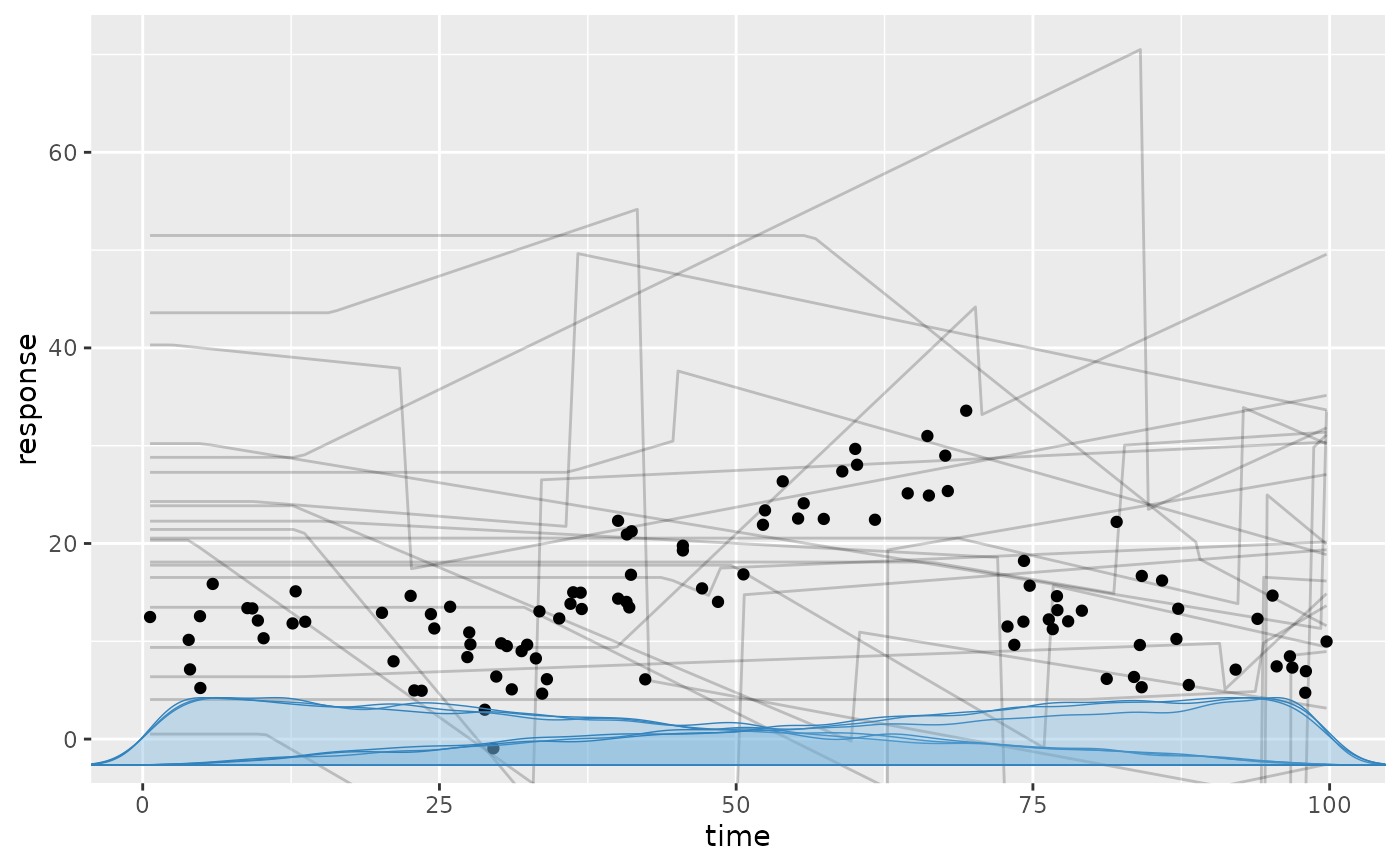
plot(demo_fit, prior = TRUE)
 # Show all priors. Default priors are added where you don't provide any
prior_summary(demo_fit)
#> # A tibble: 7 × 5
#> parameter segment dpar prior bounds
#> <chr> <int> <chr> <chr> <chr>
#> 1 cp_1 2 NA dunif(0.61863, 99.741) [0.61863, 99.741], ordered
#> 2 cp_2 3 NA dunif(0.61863, 99.741) [0.61863, 99.741], ordered
#> 3 Intercept_1 1 mu dnorm(13.825, 17.383) none
#> 4 time_2 2 mu dnorm(0, 0.62124) none
#> 5 Intercept_3 3 mu dnorm(13.825, 17.383) none
#> 6 time_3 3 mu dnorm(0, 0.62124) none
#> 7 sigma_1 1 sigma dt(0, 5.7, 3) T(0, ) [0, Inf]
# Set priors and re-run
prior = list(
Intercept_1 = 15,
time_2 = "dt(0, 2, 1) T(0, )", # t-dist slope. Truncated to positive.
cp_2 = "dunif(min(time), 80)" # change point to segment 3 before 80 (and after cp_1).
)
fit3 = mcp(model, data = data, prior = prior, seed = 42)
# Reuse coefficients in later segments using same() (e.g., Intercept_1 in segment 3)
model_same = list(
response ~ 1,
~ 0 + time,
~ same(1, as = 1) + time # Reuse Intercept_1 instead of estimating Intercept_3
)
fit_same = mcp(model_same, data = data, sample = FALSE)
# Show the JAGS model
demo_fit$jags_code
#> model {
#> # Change points
#> cp_0 = min(time)
#> cp_1 ~ dunif(cp_0, cp_3) # Flat Dirichlet on the segment lengths
#> cp_2 ~ dunif(cp_0, cp_3) # Flat Dirichlet on the segment lengths
#> cp_3 = max(time)
#> cp_order_ ~ dbern(step(cp_2 - cp_1)) # Ordered change points
#>
#> # Priors for population-level effects
#> Intercept_1 ~ dnorm(13.825120048974153, 1/(17.382500430759464)^2) # Mean intercept (rstanarm default)
#> time_2_end_ ~ dnorm(Intercept_1, 1/(0.62123709509255609*(cp_2-cp_1))^2) # Autoscaled mean coefficient (rstanarm default); sampled as the value at the segment end
#> time_2 = (time_2_end_ - (Intercept_1)) / (cp_2 - cp_1)
#> Intercept_3_end_ ~ dnorm(13.825120048974153 + time_3 * (cp_3 - cp_2), 1/(17.382500430759464)^2) # Mean intercept (rstanarm default); sampled as the value at the segment end
#> Intercept_3 = Intercept_3_end_ - (time_3 * (cp_3 - cp_2))
#> time_3 ~ dnorm(0, 1/(0.62123709509255609)^2) # Autoscaled mean coefficient (rstanarm default)
#> sigma_1 ~ dt(0, 1/(5.7)^2, 3) T(0, ) # Positive residual SD calibrated on the response scale
#>
#> # Model and likelihood
#> for (i_ in 1:length(time)) {
#> # time measured from each segment's change point
#> x_local_1_[i_] = min(time[i_], cp_1)
#> x_local_2_[i_] = min(time[i_], cp_2) - cp_1
#> x_local_3_[i_] = min(time[i_], cp_3) - cp_2
#>
#> # Formula for mu
#> link_mu_[i_] =
#> (time[i_] >= cp_0) * (time[i_] < cp_2) * inprod(rhs_matrix_[i_, c(1)], c(Intercept_1)) * 1 +
#> (time[i_] >= cp_1) * (time[i_] < cp_2) * inprod(rhs_matrix_[i_, c(2)], c(time_2)) * x_local_2_[i_] +
#> (time[i_] >= cp_2) * inprod(rhs_matrix_[i_, c(3)], c(Intercept_3)) * 1 +
#> (time[i_] >= cp_2) * inprod(rhs_matrix_[i_, c(4)], c(time_3)) * x_local_3_[i_]
#>
#> # Formula for sigma
#> link_sigma_[i_] =
#> (time[i_] >= cp_0) * inprod(rhs_matrix_[i_, c(5)], c(sigma_1)) * 1
#>
#> # Likelihood for family = gaussian()
#> mu_[i_] = link_mu_[i_]
#> sigma_[i_] = max(1e-05, link_sigma_[i_])
#> response[i_] ~ dnorm(mu_[i_], 1 / sigma_[i_]^2)
#> }
#> }
# }