From formulas to sampler code

2026-10-26

The mcp model itself is described in Understanding mcp formulas. The actual implementation is equivalent, but quite different in form. This article shows how mcp turns the segment formulas into code for the sampler, currently JAGS. You can see it as JAGS code in fit$jags_code and evaluate it in R using fit$simulate() (below).

Modeling changes in intercept

A change point is simply like an ifelse statement or multiplying with indicators (0s and 1s):

# Model parameters
x = 1:20
cp_1 = 12
Intercept_1 = 5
Intercept_2 = 10

# Ifelse version
y_ifelse = ifelse(x <= cp_1, yes = Intercept_1, no = Intercept_2)

# Indicator equivalent using dummy helpers
cp_0 = -Inf
cp_2 = Inf
y_indicator = (x > cp_0) * (x <= cp_1) * Intercept_1 +  # Between cp_0 and cp_1
              (x > cp_1) * (x <= cp_2) * Intercept_2  # Between cp_1 and cp_2

# Show it
par(mfrow = c(1,2))
plot(x, y_ifelse, main = "ifelse(x <= cp_1)")
plot(x, y_indicator, main = "(x > cp_1) * Intercept_2")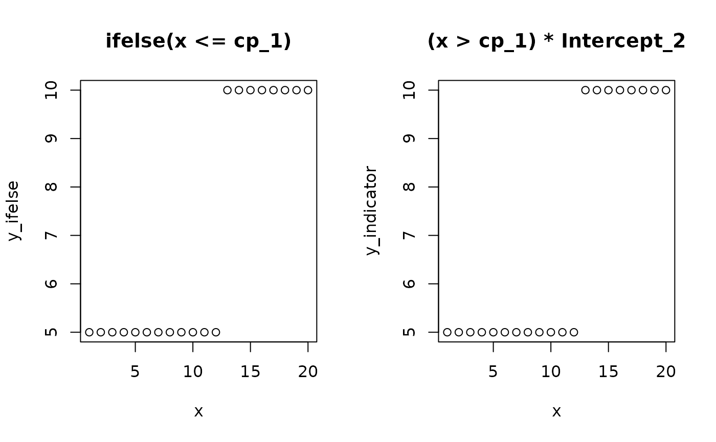

The magic of (Bayesian) MCMC sampling is that it can actually infer the change point from this simple formulation. We let mcp write the JAGS code for this simple two-plateaus model and see how it uses the indicator formulation of change points:

library(mcp)
model = list(y ~ 1, ~ 1)
fit = mcp(model, data = data.frame(y = 1:10, x = 1:10), sample = FALSE, par_x = "x")
fit$jags_code

## model {
##   # Change points
##   cp_0 = min(x)
##   cp_1 ~ dunif(cp_0, cp_2)  # Uniform within the observed range of x
##   cp_2 = max(x)
## 
##   # Priors for population-level effects
##   Intercept_1 ~ dnorm(5.5, 1/(7.5691258852437295)^2)  # Mean intercept (rstanarm default)
##   Intercept_2 ~ dnorm(5.5, 1/(7.5691258852437295)^2)  # Mean intercept (rstanarm default)
##   sigma_1 ~ dt(0, 1/(3.7)^2, 3) T(0, )  # Positive residual SD calibrated on the response scale
## 
##   # Model and likelihood
##   for (i_ in 1:length(x)) {
##     # x measured from each segment's change point
##     x_local_1_[i_] = min(x[i_], cp_1)
##     x_local_2_[i_] = min(x[i_], cp_2) - cp_1
##     
##     # Formula for mu
##     link_mu_[i_] =
##       (x[i_] >= cp_0) * (x[i_] < cp_1) * inprod(rhs_matrix_[i_, c(1)], c(Intercept_1)) * 1 + 
##       (x[i_] >= cp_1) * inprod(rhs_matrix_[i_, c(2)], c(Intercept_2)) * 1
##     
##     # Formula for sigma
##     link_sigma_[i_] =
##       (x[i_] >= cp_0) * inprod(rhs_matrix_[i_, c(3)], c(sigma_1)) * 1
## 
##     # Likelihood for family = gaussian()
##     mu_[i_] = link_mu_[i_]
##     sigma_[i_] = max(1e-05, link_sigma_[i_])
##     y[i_] ~ dnorm(mu_[i_], 1 / sigma_[i_]^2)
##   }
## }

Look at the section under the comment # Formula for mu which is the (automatically generated) model that was discussed above. Some unnecessary stuff is added to segment 1 just because it makes the code easier to generate. (x[i_] >= cp_0 when cp_0 is the smallest value of x is, of course, always true).

The section under # Change points implements the priors on the change points, explained below.

Modeling changes in slope

The mathematical definition of the piecewise model, with segments k \in \{1, \dots, K\}, change points \tau_k, intercepts \alpha_k, and slopes \beta_{k,1}, is in Understanding mcp formulas. Here is how mcp writes it in JAGS.

How mcp implements slope changes in JAGS using indicators

Bayesian MCMC samplers like JAGS cannot evaluate dynamic conditional statements (if/else) on parameters being sampled. To implement this piecewise model in JAGS, mcp uses an indicator and plateauing formulation (evaluated via Iverson brackets [A] which equal 1 when true and 0 when false).

First, mcp defines a span X_{k,i} that measures x from the change point within segment k and stays constant beyond it:

X_{1,i} = \min(x_i, \tau_1) X_{k,i} = \max\bigl(0, \min(x_i, \tau_k) - \tau_{k-1}\bigr) \quad (k \ge 2)

When x_i < \tau_{k-1}, X_{k,i} = 0 (before the segment). When \tau_{k-1} \le x_i < \tau_k, X_{k,i} = x_i - \tau_{k-1} (linear growth within the segment). When x_i \ge \tau_k, X_{k,i} = \tau_k - \tau_{k-1} (constant segment width).

For a purely joined model (list(y ~ 0 + x, ~ 0 + x)), mcp writes \eta_i as a cumulative sum of these segment spans:

\eta_i = \sum_{k=1}^K [x_i \ge \tau_{k-1}] \cdot \beta_{k,1} X_{k,i}

Because each segment’s contribution stays constant beyond its change point (\beta_{k-1,1}(\tau_{k-1} - \tau_{k-2})), joining needs no restrictions on the parameters: earlier segments provide the starting value for later segments. The expected response on the response scale is \mu_i = g^{-1}(\eta_i) via link function g(\mu_i) = \eta_i (identity for Gaussian, so \mu_i = \eta_i).

When a segment is disjoined (~ 1 + x), it introduces a new intercept \beta_{k,0} at \tau_{k-1}, and all earlier terms get the indicator [x_i < \tau_{k-1}] so they end where the disjoined segment starts. Terms that are not x-terms get the same indicator at the next change point, which is why they end there.

Let’s demonstrate this equivalence in R:

# Model parameters
x = 1:20
cp_1 = 12
slope_1 = 2
slope_2 = -1

# Ifelse version
y_ifelse = ifelse(x <= cp_1, 
            yes = slope_1 * x,
            no = cp_1 * slope_1 + slope_2 * (x - cp_1))

# Indicator version with local plateauing coordinates (pmin is vectorized min)
y_local = slope_1 * pmin(x, cp_1) + 
          (x > cp_1) * slope_2 * (x - cp_1)

# Show that both formulations are identical
par(mfrow = c(1,2))
plot(x, y_ifelse, main = "ifelse() version")
plot(x, y_local, main = "Local plateauing coordinate")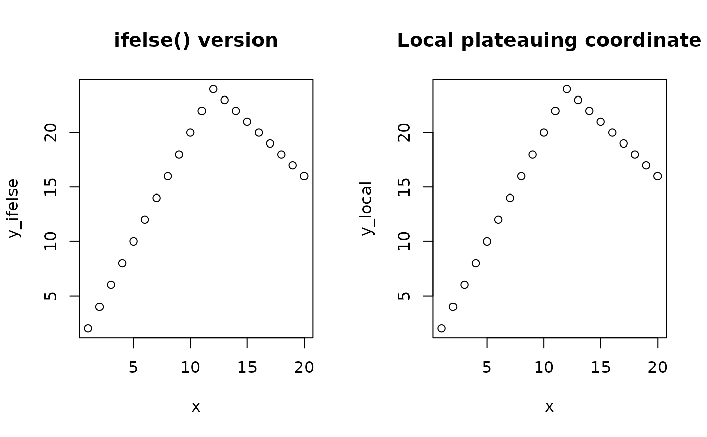

Let us see this in action:

model = list(y ~ 0 + x, ~ 0 + x)
old = options(mcp_reparam = FALSE)  # Write the plain model
fit = mcp(model, data = data.frame(y = 1:10, x = 1:10), sample = FALSE)
options(old)
fit$jags_code

## model {
##   # Change points
##   cp_0 = min(x)
##   cp_1 ~ dunif(cp_0, cp_2)  # Uniform within the observed range of x
##   cp_2 = max(x)
## 
##   # Priors for population-level effects
##   x_1 ~ dnorm(0, 1/(2.5)^2)  # Autoscaled mean coefficient (rstanarm default)
##   x_2 ~ dnorm(0, 1/(2.5)^2)  # Autoscaled mean coefficient (rstanarm default)
##   sigma_1 ~ dt(0, 1/(3.7)^2, 3) T(0, )  # Positive residual SD calibrated on the response scale
## 
##   # Model and likelihood
##   for (i_ in 1:length(x)) {
##     # x measured from each segment's change point
##     x_local_1_[i_] = min(x[i_], cp_1)
##     x_local_2_[i_] = min(x[i_], cp_2) - cp_1
##     
##     # Formula for mu
##     link_mu_[i_] =
##       (x[i_] >= cp_0) * inprod(rhs_matrix_[i_, c(1)], c(x_1)) * x_local_1_[i_] + 
##       (x[i_] >= cp_1) * inprod(rhs_matrix_[i_, c(2)], c(x_2)) * x_local_2_[i_]
##     
##     # Formula for sigma
##     link_sigma_[i_] =
##       (x[i_] >= cp_0) * inprod(rhs_matrix_[i_, c(3)], c(sigma_1)) * 1
## 
##     # Likelihood for family = gaussian()
##     mu_[i_] = link_mu_[i_]
##     sigma_[i_] = max(1e-05, link_sigma_[i_])
##     y[i_] ~ dnorm(mu_[i_], 1 / sigma_[i_]^2)
##   }
## }

We used options(mcp_reparam = FALSE) to see the plain model. By default, mcp samples some parameters on other scales, which we will return to below.

Look at the JAGS code under # x measured from each segment's change point and # Formula for mu to see this exact indicator formulation in action: x_local_1_[i_] and x_local_2_[i_] correspond to X_{1,i} and X_{2,i}, and each segment’s slope is multiplied by its indicator (e.g., (x[i_] >= cp_1)).

fitted(), predict(), log_lik(), etc. evaluate the exact same formula in R. See the model in R.

Change point priors

Each change point keeps its specified prior, but through order-restriction, the resulting “marginal” prior is different (see Working with priors). In JAGS, each change point is a node with its own prior, and one more line restricts them to ordered change points. With the default prior on two change points:

cp_0 = min(x)
cp_1 ~ dunif(cp_0, cp_3)
cp_2 ~ dunif(cp_0, cp_3)
cp_3 = max(x)
cp_order_ ~ dbern(step(cp_2 - cp_1))  # Ordered change points

Ordering: cp_order_

cp_order_ is not used anywhere else in the model. It works because mcp passes cp_order_ = 1 as data, so JAGS treats it like an observed response. Just as y[i_] ~ dnorm(...) adds the likelihood of each data point, cp_order_ ~ dbern(p) multiplies the density by the probability of observing 1, which is p. Here, p = step(cp_2 - cp_1), which is 1 if the change points are ordered and 0 otherwise. Unordered change points therefore have zero prior probability, and the sampler rejects them. This is sometimes called the “ones trick”. With three change points, the line is cp_order_ ~ dbern(step(cp_2 - cp_1) * step(cp_3 - cp_2)), and so on.

A minimum segment length, e.g., cp_2 = "dunif(cp_1 + 20, max(x))", goes in the same line as step(cp_2 - cp_1 - 20), while the node itself gets the observed range of x: cp_2 ~ dunif(cp_0, cp_3).

cp_order_ = 1 is also passed as data for prior sampling (sample = "prior"), so prior draws are ordered too. If you write your own jags_code based on fit$jags_code, mcp passes cp_order_ = 1 whenever the code contains cp_order_ ~. Without it, JAGS would sample cp_order_ like any other unknown, and the ordering would silently disappear.

Dirichlet weight: cp_weight_

dirichlet(alpha) with \alpha > 1 is the default prior multiplied by the weight \prod_k s_k^{\alpha - 1}, where s_k are the relative segment lengths (see the math).

JAGS only lets you specify priors through its built-in distributions, so it cannot multiply a prior by an arbitrary factor directly. A standard workaround is the “zeros trick”: add an observed data point whose likelihood equals the factor. mcp passes cp_weight_ = 0 as data and models it as cp_weight_ ~ dpois(lambda). The probability of observing 0 from a Poisson distribution is e^{-\lambda}, so with \lambda = -(\alpha - 1) \sum_k \log s_k, this likelihood is exactly the weight. Since s_k \le 1, \lambda \ge 0 for any \alpha \ge 1, as dpois() requires. This is also why \alpha < 1 is not supported. For example, dirichlet(2) on two change points adds this line:

cp_weight_ ~ dpois(-1 * (log((cp_1 - cp_0) / (cp_3 - cp_0)) + log((cp_2 - cp_1) / (cp_3 - cp_0)) + log((cp_3 - cp_2) / (cp_3 - cp_0))))

As with cp_order_, cp_weight_ is observed data (0), and it weights the cp_* parameters only through its likelihood. Thus, cp_weight_ is not “used” elsewhere in the JAGS code.

Initial values

The ordering must also hold for the initial values, or JAGS stops with “Observed node inconsistent with unobserved parents at initialization”. By default, all chains start at the same, equally spaced change points, moved the least possible to be inside the bounds of their priors, at least the minimum segment lengths apart, and ordered around constant change points. User-supplied initial values for change points must be ordered.

Reparameterizations

By default (options(mcp_reparam = TRUE)), fit$jags_code samples some coefficients via auxiliary nodes, ending in _mid_, _end_, or _rise_. This is a reparameterization, not a new model: the priors, and hence the posteriors, are exactly those of the plain model. Only the sampling becomes faster and converges more reliably. options(mcp_reparam = FALSE) shows the plain model.

Like most Gibbs samplers, JAGS updates one parameter at a time while holding the others fixed. In the plain model, an intercept is the value at the start of its segment, and a joined segment starts where the previous segment ended. So if JAGS moves a change point \tau_k while holding the slopes fixed, the lines of segment k+1, and of all later joined segments, shift up or down. Such moves fit the data badly and are mostly rejected, so the change points and the coefficients must creep along together, which mixes slowly. With reparameterizations, mcp instead samples quantities that stay in place when a change point moves.

All reparameterizations follow from one fact: if a coefficient \beta has a location-scale prior, e.g., \beta \sim \text{Normal}(m, s), then for any shift a and scale b > 0,

u = a + b \beta \quad \sim \quad \text{Normal}(a + b m, \; b s).

So JAGS can sample u with this prior and derive \beta = (u - a) / b, and \beta has exactly its original prior. This holds when a and b depend on other parameters, such as change points and other coefficients, because the prior on \beta given those parameters is unchanged. Here is what mcp samples, with segment widths w_k = \tau_k - \tau_{k-1} and \alpha_k being the value where segment k starts:

Coefficient	Sampled u	a	b
Segment 1 intercept \beta_{1,0}	Value at c	\beta_{1,1} c	1
Joined slope \beta_{k,1}	Value at segment end e_k = \alpha_k + \beta_{k,1} w_k	\alpha_k	w_k
Joined I(x^2) term \beta_{k,2}	Rise \beta_{k,2} w_k^2	0	w_k^2
Disjoined intercept \beta_{k,0}	Value at segment end e_k = \beta_{k,0} + \beta_{k,1} w_k	\beta_{k,1} w_k	1

We will go through them one by one for this model with x = 1:100:

model = list(
  y ~ 1 + x,  # x_1 = 17.5
  ~ 0 + x + I(x^2),
  ~ 1 + x
)

The same rules apply to distributional parameters such as sigma(1 + x).

Segment 1 intercept: _mid_

# mcp_reparam = FALSE
Intercept_1 ~ dnorm(0 - x_1 * 1, 1/(2.4)^2)  # JAGS uses dnorm(mean, precision) with precision = 1/SD^2. Here SD = 2.4

# mcp_reparam = TRUE
Intercept_1_mid_ ~ dnorm(0 - x_1 * 1 + x_1 * (17.5), 1/(2.4)^2)
Intercept_1 = Intercept_1_mid_ - (x_1 * (17.5))
x_1 ~ dnorm(0, 1/(0.084)^2)

JAGS samples the value of segment 1 at the fixed point c = \min(x) + (\max(x) - \min(x)) / (2K), which is the midpoint of segment 1 under the default prior on change points. Here, c = 1 + (100 - 1) / (2 \cdot 3) = 17.5. Intercept_1 is derived from it. Like centering x in ordinary regression, this makes the intercept and slope less correlated. In the plain model, the intercept is the value at x = 0, which can be far from the data. Then every change in the slope must be met by a large opposite change in the intercept, and a sampler that updates one at a time moves in tiny steps.

This is the same model because u = \beta_{1,0} + \beta_{1,1} c is a mere shift (a = \beta_{1,1} c, b = 1), so the prior on Intercept_1 is unchanged. The prior on Intercept_1 is on the value at \min(x) = 1, hence the - x_1 * 1 in the prior mean. A shift moves bounds by a too, so this also works for truncated and dunif() priors.

Joined slope: _end_

# mcp_reparam = FALSE
x_2 ~ dnorm(0, 1/(0.084)^2)  # SD = 0.084

# mcp_reparam = TRUE
x_2_end_ ~ dnorm(Intercept_1 + x_1 * cp_1, 1/(0.084*(cp_2-cp_1))^2)  # SD = 0.084 * (cp_2 - cp_1)
x_2 = (x_2_end_ - (Intercept_1 + x_1 * cp_1)) / (cp_2 - cp_1)

JAGS samples the value at the end of segment 2, e_2, and derives the slope x_2 from it. In the plain model, moving \tau_1 shifts segment 2 up or down, together with all later joined segments. Now, moving \tau_1 pivots segment 2 around its end, so later segments stay in place.

This is the same model because the value at the segment end is the starting value plus the slope times the segment width, e_k = \alpha_k + \beta_{k,1} w_k. Here, \alpha_2 = Intercept_1 + x_1 * cp_1 and w_2 = cp_2 - cp_1. With a = \alpha_k and b = w_k, the prior on e_k is centered on \alpha_k + w_k m with SD w_k s, as in the JAGS code above. The derived slope x_2 has its original prior, whatever the change points and the earlier coefficients are.

Further joined x-terms: _rise_

# mcp_reparam = FALSE
xE2_2 ~ dnorm(0, 1/(0.00082)^2)  # SD = 0.00082

# mcp_reparam = TRUE
xE2_2_rise_ ~ dnorm(0, 1/(0.00082*(cp_2-cp_1)^2)^2)  # SD = 0.00082 * (cp_2 - cp_1)^2
xE2_2 = xE2_2_rise_ / (cp_2 - cp_1)^2

Further x-terms in joined segments, here I(x^2), are sampled as their rise over the segment, \beta_{k,2} w_k^2. This is how much the term adds to the value at the segment end. Together with the slope’s _end_ node, the value at the segment end then stays in place when a change point moves, so later joined segments stay in place too.

This is the same model because the rise is a mere scaling (a = 0, b = w_k^2), so the prior SD is scaled by w_k^2 in the JAGS code above, and xE2_2 has its original prior.

Disjoined intercept: _end_

# mcp_reparam = FALSE
Intercept_3 ~ dnorm(0, 1/(2.4)^2)  # SD = 2.4

# mcp_reparam = TRUE
Intercept_3_end_ ~ dnorm(0 + x_3 * (cp_3 - cp_2), 1/(2.4)^2)
Intercept_3 = Intercept_3_end_ - (x_3 * (cp_3 - cp_2))
x_3 ~ dnorm(0, 1/(0.084)^2)

JAGS samples the value at the end of segment 3, e_3, and derives Intercept_3 from it. In the plain model, Intercept_3 is the value where segment 3 starts, so moving \tau_2 while holding Intercept_3 and x_3 fixed shifts the whole line of segment 3 sideways. Now, segment 3’s line, e_3 + \beta_{3,1}(x - \tau_3), does not depend on \tau_2 at all.

This is the same model because e_k = \beta_{k,0} + \beta_{k,1} w_k is a mere shift (a = \beta_{k,1} w_k, b = 1), so the prior on Intercept_3 is unchanged.

When mcp does not reparameterize

mcp only reparameterizes its default dnorm() and dt() priors, and for the segment-1 intercept also truncated and dunif() priors. User-specified priors are sampled unchanged, and so are coefficients in segments that start or end at group-level change points, where the segment widths differ between groups.

The model in R

fitted(), predict(), log_lik(), loo(), and plot() evaluate the same model in R. Internally, the formula in fit$jags_code and the R evaluation are written from the same table of terms, so the two always agree. To evaluate the model for chosen parameter values, use fit$simulate(). For the joined slopes above, it reproduces the indicator version:

y_mcp = fit$simulate(fit, data.frame(x = 1:20), cp_1 = 12, x_1 = 2, x_2 = -1, sigma_1 = 1, .type = "fitted")
all.equal(as.numeric(y_mcp), y_local)

## [1] TRUE

The priors and reparameterizations are not part of the R evaluation. The likelihood is in fit$family$r, e.g., fit$family$r$log_lik and fit$family$r$rng.