Group-level (random) effects in mcp

mcp supports group-level effects (also called random effects) in both the predictor and change-point parts of a formula. The syntax follows lme4 and brms: (1|group) specifies a group-level intercept, (factor||group) specifies independent group coefficients, fixef() reports population-level effects, and ranef() reports group-level deviations.

This article in brief:

Predictor and change-point group-level effects
How group-level effects persist across segments
How to simulate group-level change-point deviations
Get posteriors using ranef(fit)
Plot using plot(fit, facet_by="my_group") and plot_pars(fit, pars = "group", type = "dens_overlay", ncol = 3).
How group-specific change points are kept in range and ordered.
The article on modeling standard deviation via sigma() contains another group-level change-point example.

library(mcp)
future::plan(future::multisession, workers = 3)
set.seed(42)  # Make the script deterministic

Specifying group-level change points

You specify group-level effects using the familiar lmer and brms syntax (1|group). In the cp part, this models a group-specific deviation from the population-level change point. For example:

model = list(
  y ~ 1,  # Intercept_1
  1 + (1|id) ~ 0 + x  # cp_1, cp_1_sd, cp_1_id[i]
)

You can have multiple group-level change points, but they must use the same grouping factor so their realized locations can be ordered within each group:

model = list(
  y ~ 1,  # Intercept_1
  1 + (1|id) ~ 0 + x,  # cp_1, cp_1_sd, cp_1_id[i]
  1 + (1|id) ~ 0,      # cp_2, cp_2_sd, cp_2_id[i]
  (1|id) ~ 1           # cp_3 (implicit), cp_3_sd, cp_3_id[i]
)

For change point i and group g, the hierarchy is

\kappa_{ig} \sim \operatorname{Normal}(cp_i, cp_{i,\mathrm{sd}}), \qquad cp_{i,\mathrm{id}[g]} = \kappa_{ig} - cp_i,

where \kappa_{ig} is the group-specific location. Thus cp_i_id[g] is the reported deviation and cp_i_sd is the latent normal scale. The deviations are not forced to sum to zero.

The hierarchy is subject to x_{\min} < \kappa_{1g} < \cdots < \kappa_{Kg} < x_{\max}. Thus, if adjacent change points both vary, their group-specific locations are ordered against each other—not against the adjacent population change point. Internally, JAGS samples \kappa_{ig} directly for efficiency.

Unlike predictor group-level effects, a change-point group effect applies only to the boundary where it is written. There is no carry-over as there is for group-level effects on RHS.

Predictor group-level effects

The same syntax in the predictor part gives each group a deviation from the population-level intercept:

model = list(
  y ~ 1 + (1|id),  # Starts group-level intercept
  ~ 0 + x,         # Group-level intercept persists here
  ~ 1 + (0|id)     # 0 Turns it off
)

Here, the group-level intercept introduced in segment 1 also applies in segment 2. A later (1|id) would replace it from that segment onward, while (0|id) turns it off, as in segment 3 above. Persistence is tracked separately for each grouping factor and distributional parameter. Read more on carry-over rules between segments in the article on formulas.

Use || for independent group-level slopes and factor coefficients:

model = list(
  y ~ 1 + condition + (condition||id),
  ~ 0 + x
)

With the default treatment coding, (condition||id) contains a group-level intercept and one group-level deviation for each non-reference contrast of condition. (0 + condition||id) instead gives each factor level its own group-level coefficient. Similarly, (1 + z||id) specifies independent group-level intercepts and slopes on a numeric predictor z. Each coefficient has its own population-level SD.

The population-level and group-level formulas need not contain the same coefficients. For example, y ~ 1 + (0 + condition||id) has a population-level intercept but only group-specific condition coefficients.

Group-level intercepts also work inside distributional formulas:

model = list(
  y ~ 1 + (1|id) + sigma(1 + (1|id))
)

This model has group-level deviations in both the conditional mean and log-SD. The || syntax works inside distributional formulas too, for example sigma(1 + (condition||id)).

A later predictor group-level term for the same distributional parameter and grouping factor replaces the entire earlier block. Thus, if (condition||id) is followed in a later segment by (1||id), only the new intercept deviation applies from that segment onward. (0|id) turns the block off.

Multi-coefficient terms with |, such as (1 + x|id), would imply correlated group coefficients and are not yet supported; use (1 + x||id) for independent coefficients. Group-level terms inside ar() and ma() are also not supported.

Unlike change-point deviations, predictor deviations are not constrained to sum exactly to zero. They have an ordinary mean-zero hierarchical normal distribution, matching multilevel regression in lme4 and brms. For example, (1|id) in segment 1 creates the deviation vector Intercept_1_id and its population-level SD parameter Intercept_1_id_sd. (condition||id) additionally creates names such as conditionB_1_id and conditionB_1_id_sd; inside sigma(), the corresponding names start with sigma.

Simulating group-level change points

Let us simulate group-specific deviations in the change point between a plateau and a slope:

model = list(
  y ~ 1,  # Intercept_1
  1 + (1|id) ~ 0 + x  # cp_1, cp_1_sd, cp_1_id[i]
)

This follows the same interface as predictor group-level effects: supply the population-level SD and fit$simulate() draws one deviation per group and centers them exactly on zero.

library(dplyr, warn.conflicts = FALSE)
group_levels = c("Clark", "Louis", "Batman", "Batgirl", "Spiderman", "Jane")
df = data.frame(
  x = runif(length(group_levels) * 30, 0, 100),  # 30 data points for each
  id = rep(group_levels, each = 30),  # the group names
  y = 1
)
empty = mcp(model, data = df, sample = FALSE)

set.seed(42)
df$y = empty$simulate(empty, df,
  # Population-level:
  Intercept_1 = 20, x_2 = 0.5, cp_1 = 50, sigma = 2,
  
  # Generate exactly centered group-level deviations with this SD
  cp_1_sd = 15)

head(df)

##          x    id        y
## 1 91.48060 Clark 31.74661
## 2 93.70754 Clark 32.40289
## 3 28.61395 Clark 19.78775
## 4 83.04476 Clark 29.28600
## 5 64.17455 Clark 19.81068
## 6 51.90959 Clark 24.03685

For models with multiple group-level change points, all deviations are drawn once and then checked for ordering. An unordered draw produces an error; fit$simulate() does not redraw, sort, or clip the change points. The result:

library(ggplot2)
ggplot(df, aes(x=x, y=y)) + 
  geom_point() +
  facet_wrap(~id)

Summarise and plot group-level effects

Fitting the model is simple:

fit = mcp(model, data = df, seed = 42)

If we just use plot(fit), we would see all points in one plot. We want to facet by id, so:

set.seed(42)
plot(fit, facet_by = "id")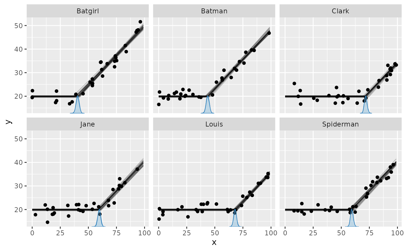

It seems that mcp recovered the group-specific change points well. There is a lot of information in these data because the population-level intercept and slopes on either side of the change point are shared across participants (id).

summary(fit) (or fixef(fit)) returns posterior summaries for the population-level effects. To get the group-level deviations (random effects), use:

mcp::ranef(fit)

##             variable       mean       sd     lower    upper     rhat ess_bulk ess_tail       sim match
## 1   cp_1_id[Batgirl]   7.748753 23.56258 -31.85555 58.85708 1.001548     4745     5882 14.315858    OK
## 2    cp_1_id[Batman] -16.906485 23.54159 -56.42552 34.31066 1.001206     4656     5862 -8.463936    OK
## 3     cp_1_id[Clark]  12.532440 23.55908 -27.01466 63.70903 1.001393     4698     5954 20.518845    OK
## 4      cp_1_id[Jane]  -6.806863 23.53981 -46.22738 44.38053 1.001252     4698     6116  0.715170    OK
## 5     cp_1_id[Louis]  18.201298 23.56281 -21.31165 69.60913 1.001186     4691     6085 22.900143    OK
## 6 cp_1_id[Spiderman]  -1.480419 23.54962 -40.98176 49.48032 1.001462     4675     5991  5.438742    OK

Inspecting the sim and match columns, we see that they recovered the simulation parameters well.

Prediction methods include all group-level effects by default. Set varying = FALSE for population-only predictions, varying = "cp" for all group-level effects in the cp part, varying = "predictor" for predictor-side group-level effects, or supply an exact name such as varying = "cp_1_id". ranef(fit) deliberately remains simple and returns all group-level effects.

Good convergence is not always as obvious as in this example. While plot_pars(fit) shows population-level parameters only, you can select the group-level deviations with "group":

set.seed(42)
plot_pars(fit, pars = "group", type = "trace", ncol = 3, nvariable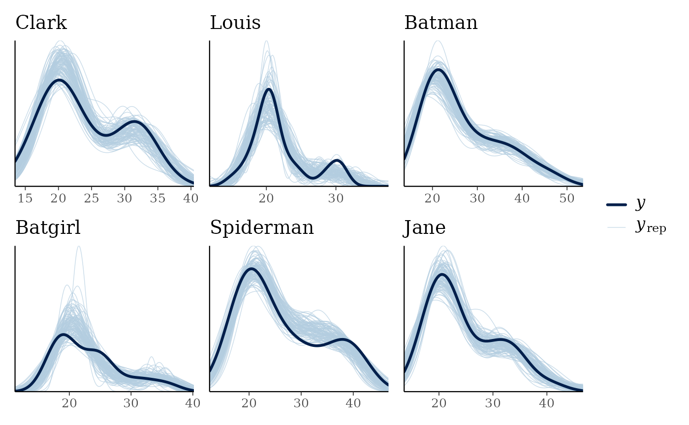s = NULL)

The ncol argument controls the number of columns. Group-level effects often have many levels, so this is useful for viewing all deviations.

Using pars = "group" plots all group-level deviations. To select one group-level effect, use a regular expression in regex_pars; for example, ^ anchors the start of a parameter name:

set.seed(42)
plot_pars(fit, regex_pars = "^cp_1_id", type = "dens_overlay", ncol = 2, nvariable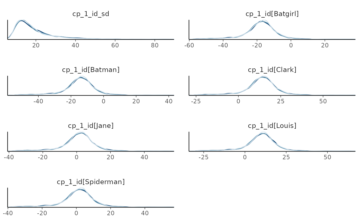s = NULL)

You can also do posterior predictive checking with facets. I think that for the relatively univariate models supported as of mcp 0.3, this does not add much new information over and above plot(fit, facet_by = "id"), but it’s a standard assessment that many will be acquainted with:

set.seed(42)
pp_check(fit, facet_by = "id")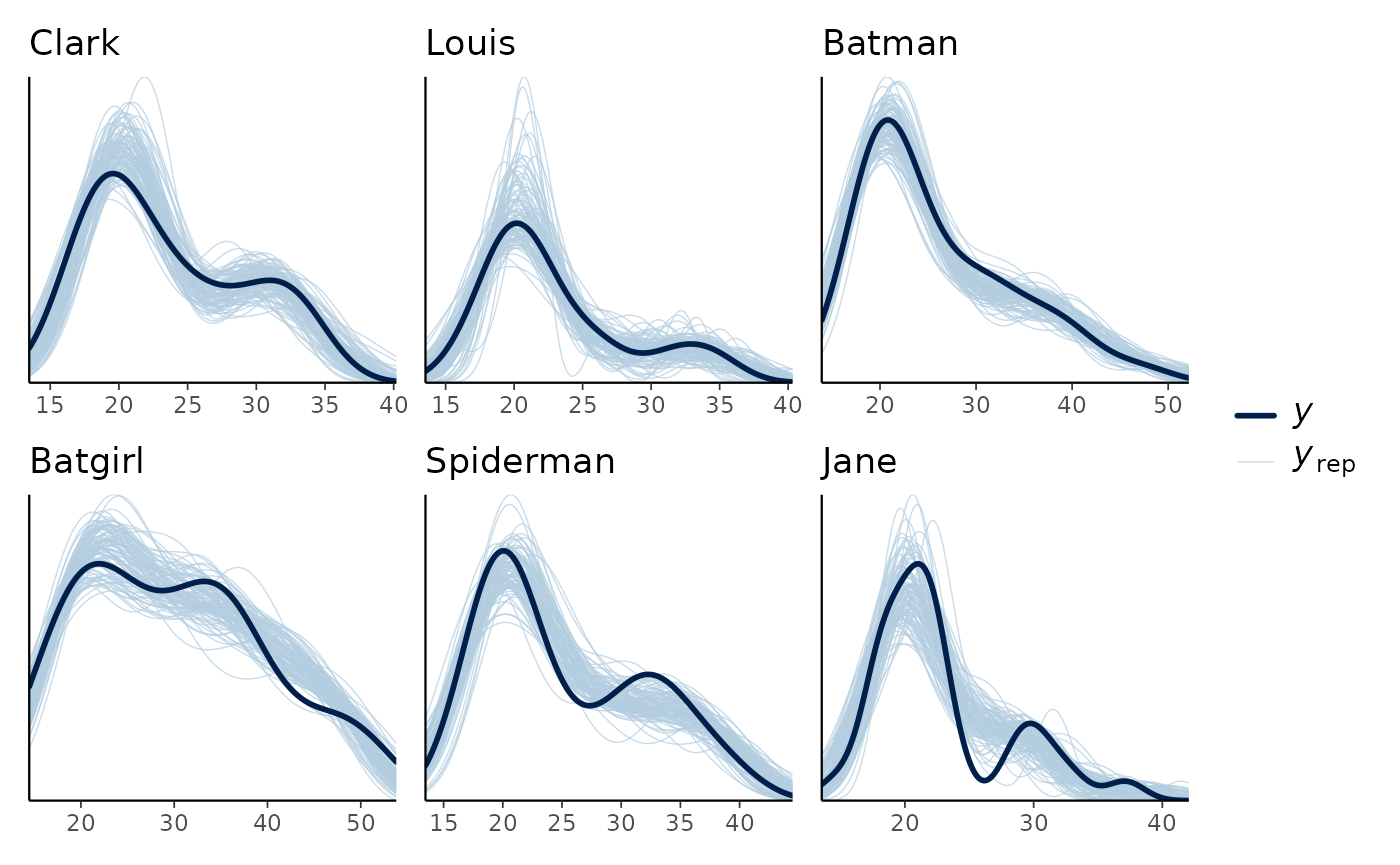

Priors for group-level effects

You can see the priors of the model like this:

prior_summary(fit)

## # A tibble: 6 × 5
##   parameter   segment dpar  prior                                               bounds                        
##   <chr>         <int> <chr> <chr>                                               <chr>                         
## 1 cp_1              2 cp    dirichlet(alpha = 1)                                [min(x), max(x)]              
## 2 cp_1_sd           2 cp    normal(mean = 0, sd = 197.7306)                     [0, Inf]                      
## 3 cp_1_id           2 cp    normal(mean = 0, sd = cp_1_sd)                      [min(x) - cp_1, max(x) - cp_1]
## 4 Intercept_1       1 mu    student_t(df = 3, location = 21.7, scale = 4.6)     none                          
## 5 x_2               2 mu    student_t(df = 3, location = 0, scale = 0.04652796) none                          
## 6 sigma_1           1 sigma student_t(df = 3, location = 0, scale = 4.6)        [0.001, Inf]

cp_1_sd is the latent normal scale governing the cp_1_id deviations. Unlike predictor group-level effects, change-point locations are also constrained to remain in range and ordered within each group.

JAGS code

Here is the JAGS code for the model used in this article:

fit$jags_code