Variance change points and other distributional parameters

mcp supports distributional regression, where any parameter of a response distribution can be regressed on predictors and have change points across segments. In standard regression, formulas model only the conditional mean mu(), where the expected response on the response scale relates to the linear predictor via link function g(\mu_i) = \eta_i (\mu_i = g^{-1}(\eta_i)). Distributional regression extends this by allowing formulas for distributional parameters such as residual standard deviation (sigma), negative-binomial overdispersion (shape) - and auxiliary parameters for time-series autocorrelation (ar / ma) - on their respective link scales.

In mcp, a distributional parameter (dpar) is anything with its own segmented linear predictor: mu, sigma, shape, and each AR/MA lag (ar1, ar2, ma1, …). Strictly, AR/MA lags are not parameters of the response distribution, but they are modeled the same way. This is what the dpar argument and column refer to throughout mcp, e.g., fitted(fit, dpar = "sigma"), plot_dpar(fit, "ar1"), fixef(fit, dpar = "ar1"), and mcp_pars(fit)$dpar.

Here, we exemplify regression on the standard deviation sigma. A plateau mean with an increasing standard deviation can be written as y ~ 1 + sigma(1 + x). Read more about mcp formulas here.

Priors for distributional parameters

Aligning with brms convention, without an explicit sigma() formula, the default is the intercept-only prior dt(0, max(2.5, mad(y)), 3) T(0, ) directly on the residual SD, i.e., an identity link. The response-calibrated scale adapts to the units of y, with a minimum of 2.5 to avoid an accidentally narrow prior.

With an explicit sigma() formula, the intercept instead defaults to dt(0, 2.5, 3) on log-SD, as in brms. Contrasts use the same prior, and slopes are scaled by the predictor’s SD, dt(0, 2.5 / sd(column), 3). Read more.

Simple example: a change in standard deviation

Let us model a simple change in residual standard deviation with a plateau mean:

library(mcp)
future::plan(future::multisession, workers = 3)

model = list(
  y ~ 1,  # sigma(1) is implicit in the first segment
  ~ 0 + sigma(1)  # a new intercept on sigma, but not on the mean
)

We can simulate data with an abrupt change from a low to a high residual standard deviation at x = 50:

df = data.frame(x = 1:100, y = 1)
empty = mcp(model, data = df, sample = FALSE, par_x = "x")

df$y = empty$simulate(
  empty, df, 
  cp_1 = 50, Intercept_1 = 20, 
  sigma_Intercept_1 = log(5), sigma_Intercept_2 = log(20))

head(df)

##   x        y
## 1 1 23.26959
## 2 2 20.09526
## 3 3 10.75248
## 4 4 19.33618
## 5 5 14.00591
## 6 6 13.35129

Now we fit the model to the simulated data.

fit = mcp(model, data = df, par_x = "x")

We plot a posterior predictive interval to show the effect of the changing standard deviation, which is not immediately visible in the default plot of the expected response:

plot(fit, interval = "predict")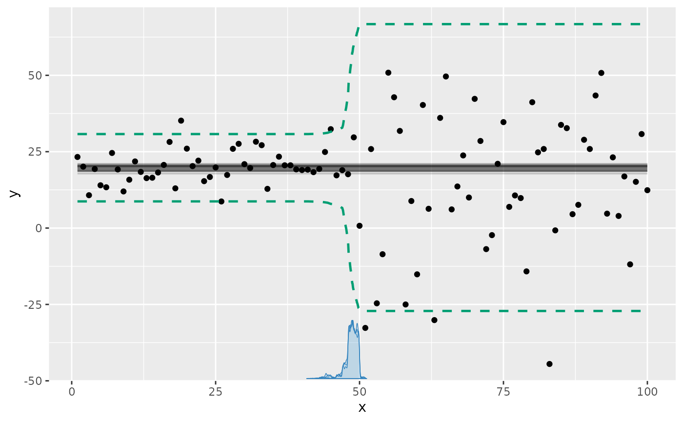

We can see all parameters are well recovered (compare sim to mean) despite poor rhat and ESS. Like the other parameters, the sigma coefficients are named after the segment where they are included. There will always be a sigma_Intercept_1 because sigma is required by the likelihood.

summary(fit)

## Family: gaussian
## Links: mu = identity; sigma = log
## Draws: 9000 (3 chains with iter = 3000)
## Segments:
##   1: y ~ 1
##   2: ~ 0 + sigma(1)
## 
## Change point parameters:
##          parameter   mean    sd  lower  upper rhat ess_bulk ess_tail    sim match
##  cp_1              48.6   1.2   44.7   50.0   1.00     2380      795 50.0      OK
## 
## Population-level parameters:
##          parameter   mean    sd  lower  upper rhat ess_bulk ess_tail    sim match
##  Intercept_1       19.75  0.77  18.25  21.29  1.00     8093     8386 20.00     OK
##  sigma_Intercept_1  1.70  0.11   1.49   1.92  1.00     4749     4707  1.61     OK
##  sigma_Intercept_2  3.156 0.099  2.971  3.358 1.00     5444     4697  2.996    OK

Advanced example

We can model changes in sigma alone or together with changes in the mean. The following deliberately complex model demonstrates that flexibility:

model = list(
  # 1. Increasing standard deviation.
  y ~ 1 + sigma(1 + x),  # Intercept_1, sigma_Intercept_1, sigma_x_1
  
  # 2. Abrupt change in mean and standard deviation.
  ~ 1 + sigma(1),  # At cp_1: Intercept_2, sigma_Intercept_2
  
  # 3. Joined slope on mean; log-SD changes as a second-order polynomial.
  ~ 0 + x + sigma(0 + x + I(x^2)),  # At cp_2: x_3, sigma_x_3, sigma_xE2_3
  
  # 4. Continue slope on mean, but plateau standard deviation (no sigma() term).
  ~ 0 + same(x)  # At cp_3: reuse x_3; sigma joined
)

Notice a few things here:

same(x) ensures that the mean slope remains constant between segment 3 and 4. So only sigma changes there. Reusing the slope effectively removes the change point in the mean (read more about formulas in mcp).
Segment 4: sigma is required by the likelihood, so it cannot be turned off. A segment that does not include sigma() is joined, so the log-SD plateaus here.

In general, the log-SD parameters are named sigma_[normalname], where “normalname” is the usual parameter names in mcp (see more here). For example, the log-SD intercept in segment 2 is sigma_Intercept_2 and the log-SD slope on x in segment 3 is sigma_x_3. In models without sigma(), the residual SD itself is simply sigma_1.

Simulate data

We simulate some data from this model, setting all parameters. As always, we can make an empty fit (sample = FALSE) to get fit$simulate, which is useful for simulation and predictions from this model.

# Set up model
df = data.frame(x = 1:200, y = 1)
empty = mcp(model, data = df, sample = FALSE)

# Simulate data
df$y = empty$simulate(
  empty, df,
  cp_1 = 50, cp_2 = 80, cp_3 = 140,
  Intercept_1 = -20, Intercept_2 = 0,
  sigma_Intercept_1 = log(1), sigma_x_1 = log(2) / 15,
  sigma_Intercept_2 = log(4),
  sigma_x_3 = 0.03,
  sigma_xE2_3 = 0.00015,
  x_3 = 0.8
)

Fit it and inspect results

Fit it:

fit = mcp(model, data = df, diagnostics = FALSE)

Plotting a posterior predictive interval is an intuitive way to see how the residual standard deviation is estimated:

plot(fit, interval = "predict")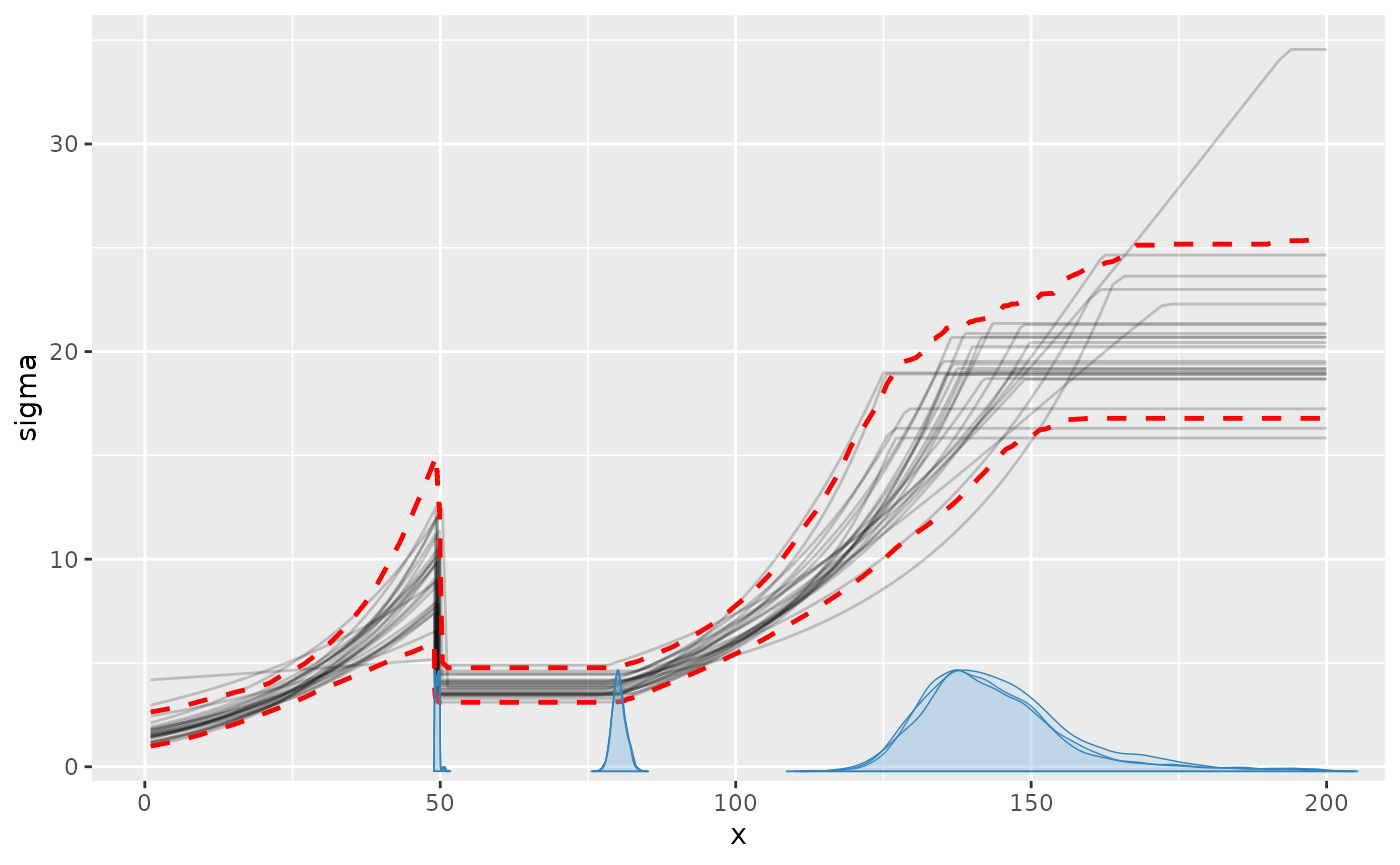

We can also plot sigma itself using plot_dpar(). Now the y-axis is the residual SD:

plot_dpar(fit, dpar = "sigma", interval = "fitted")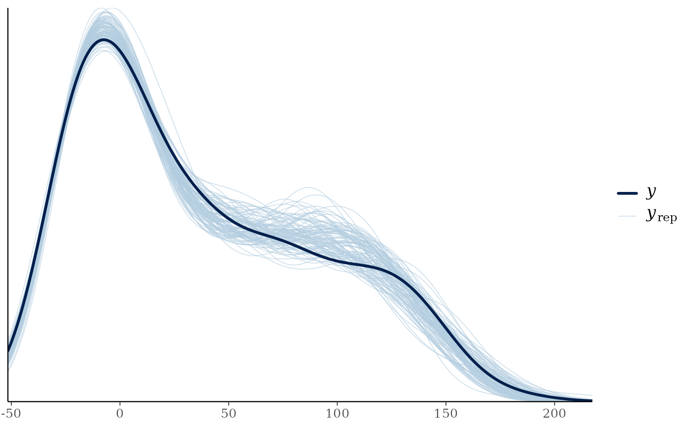

summary(fit) shows that the parameters are well recovered and a posterior predictive check (pp_check(fit)) looks good too. The last change point is estimated with greater uncertainty than the others because its only signal is a stop in standard-deviation growth.

summary(fit)

## Family: gaussian
## Links: mu = identity; sigma = log
## Draws: 9000 (3 chains with iter = 3000)
## Segments:
##   1: y ~ 1 + sigma(1 + x)
##   2: ~ 1 + sigma(1)
##   3: ~ 0 + x + sigma(0 + x + I(x^2))
##   4: ~ 0 + same(x)
## 
## Change point parameters:
##          parameter      mean      sd     lower     upper rhat ess_bulk ess_tail       sim match
##  cp_1               49.36    0.56     48.13     50.42    1.00     3290     2903  50.00       OK
##  cp_2               82.6     1.6      79.3      85.7     1.00     2653     3564  80.0        OK
##  cp_3              143.4     7.2     130.5     158.0     1.05       74      105 140.0        OK
## 
## Population-level parameters:
##          parameter      mean      sd     lower     upper rhat ess_bulk ess_tail       sim match
##  Intercept_1       -19.74    0.38    -20.48    -18.95    1.00     7479     7912 -20.00       OK
##  Intercept_2         0.58    0.63     -0.67      1.82    1.00     4927     6198   0.00       OK
##  x_3                 0.861   0.058     0.749     0.974   1.00     5747     7346   0.800      OK
##  sigma_Intercept_1   0.22    0.22     -0.19      0.69    1.00     4477     4873   0.00       OK
##  sigma_x_1           0.0388  0.0079    0.0234    0.0543  1.00     4101     4972   0.0462     OK
##  sigma_Intercept_2   1.28    0.12      1.07      1.52    1.01     1378     3438   1.39       OK
##  sigma_x_3           0.0425  0.0094    0.0222    0.0609  1.09       28       66   0.0300     OK
##  sigma_xE2_3        -0.00000 0.00018  -0.00033   0.00047 1.11       25       52   0.00015    OK

pp_check(fit)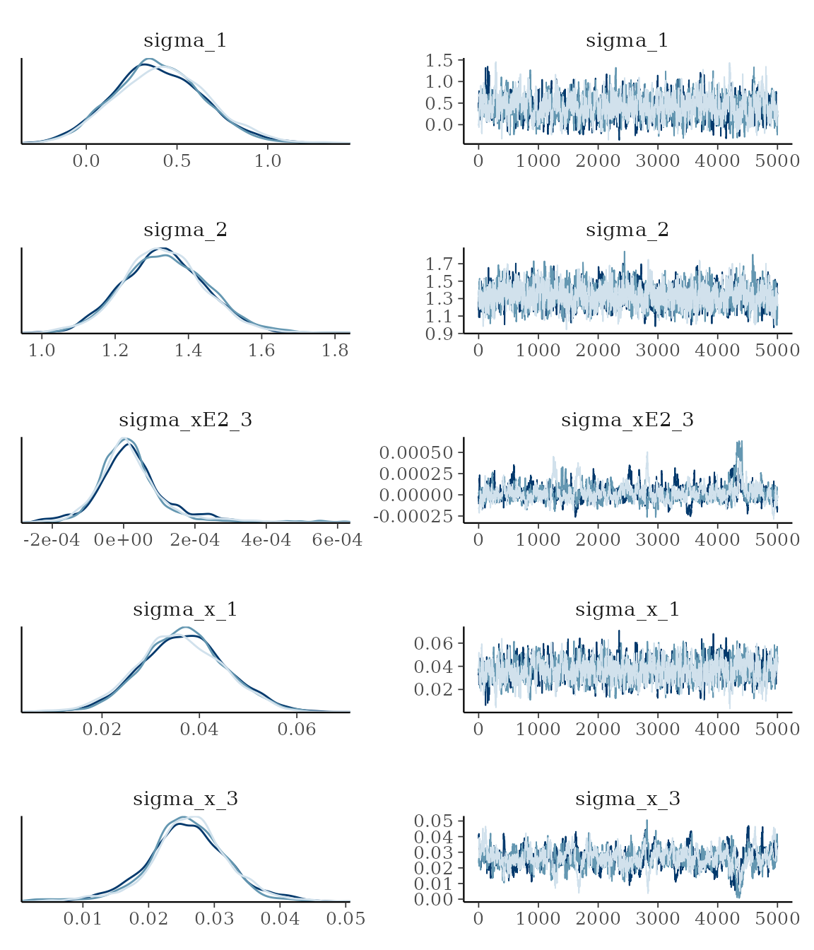

The low ESS for sigma in segment 3 reveals some unidentifiability concerning whether the variance increase is driven by a linear (sigma_x_3) or quadratic term (sigma_xE2_3). This spills over to a lower ESS for cp_3 too. Other coefficients seem to be reasonably recovered. This is why I set diagnostics = FALSE to quiet warnings since this is just a demonstration.

Let us verify this by taking a look at the posteriors and trace. For now, we just look at the sigmas:

plot_pars(fit, regex_pars = "sigma_")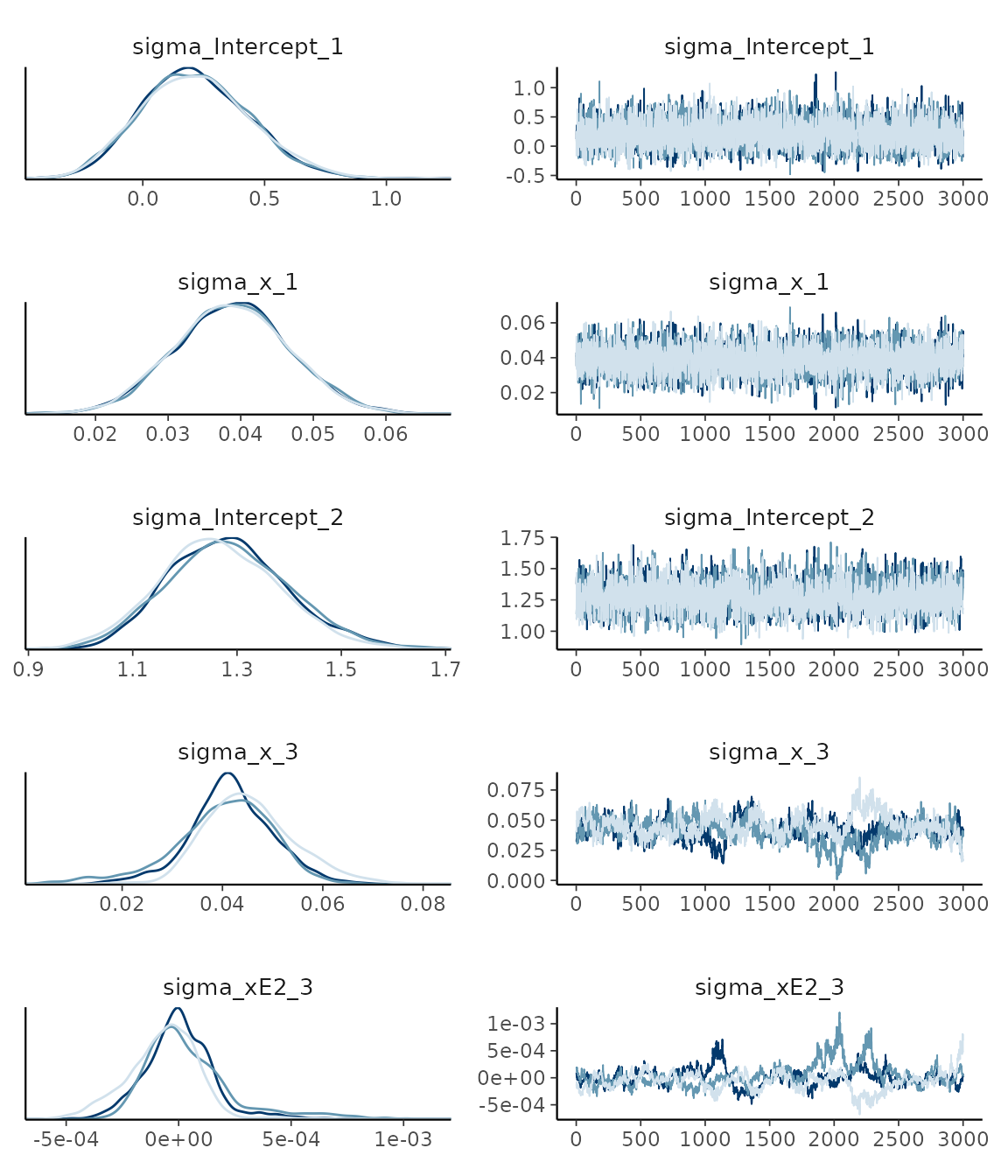

This confirms the impression from rhat, ess_bulk, and ess_tail. Read more about tips, tricks, and debugging.

JAGS code for distributional parameters

Printing the underlying JAGS code, you can see that the regression model is the same for the mean mu (see under “# Formula for mu”) and the standard deviation sigma (see under “# Formula for sigma”).

This is explained more in Understanding mcp formulas.

fit$jags_code

## model {
##   # Change points
##   cp_0 = min(x)
##   cp_1 ~ dunif(cp_0, cp_4)  # Flat Dirichlet on the segment lengths
##   cp_2 ~ dunif(cp_0, cp_4)  # Flat Dirichlet on the segment lengths
##   cp_3 ~ dunif(cp_0, cp_4)  # Flat Dirichlet on the segment lengths
##   cp_4 = max(x)
##   cp_order_ ~ dbern(step(cp_2 - cp_1) * step(cp_3 - cp_2))  # Ordered change points
## 
##   # Priors for population-level effects
##   Intercept_1 ~ dnorm(26.268121747257734, 1/(118.97849793160449)^2)  # Mean intercept (rstanarm default)
##   Intercept_2 ~ dnorm(26.268121747257734, 1/(118.97849793160449)^2)  # Mean intercept (rstanarm default)
##   x_3_end_ ~ dnorm(Intercept_2, 1/(2.055635353724206*(cp_3-cp_2))^2)  # Autoscaled mean coefficient (rstanarm default); sampled as the value at the segment end
##   x_3 = (x_3_end_ - (Intercept_2)) / (cp_3 - cp_2)
##   sigma_Intercept_1_mid_ ~ dt(-sigma_x_1 * 1 + sigma_x_1 * (25.875), 1/(2.5)^2, 3)  # Weakly regularizing modeled log-SD intercept; on the value at min(x); sampled as the value at the expected midpoint of segment 1
##   sigma_Intercept_1 = sigma_Intercept_1_mid_ - (sigma_x_1 * (25.875))
##   sigma_x_1 ~ dt(0, 1/(0.043193421279068007)^2, 3)  # Regularizing log-SD coefficient scaled by the predictor SD
##   sigma_Intercept_2 ~ dt(0, 1/(2.5)^2, 3)  # Weakly regularizing modeled log-SD intercept
##   sigma_x_3_end_ ~ dt(sigma_Intercept_2, 1/(0.043193421279068007*(cp_3-cp_2))^2, 3)  # Regularizing log-SD coefficient scaled by the predictor SD; sampled as the value at the segment end
##   sigma_x_3 = (sigma_x_3_end_ - (sigma_Intercept_2)) / (cp_3 - cp_2)
##   sigma_xE2_3_rise_ ~ dt(0, 1/(0.0002100945749551876*(cp_3-cp_2)^2)^2, 3)  # Regularizing log-SD coefficient scaled by the predictor SD; sampled as the rise over the segment
##   sigma_xE2_3 = sigma_xE2_3_rise_ / (cp_3 - cp_2)^2
## 
##   # Model and likelihood
##   for (i_ in 1:length(x)) {
##     # x measured from each segment's change point
##     x_local_1_[i_] = min(x[i_], cp_1)
##     x_local_2_[i_] = min(x[i_], cp_2) - cp_1
##     x_local_3_[i_] = min(x[i_], cp_3) - cp_2
##     x_local_4_[i_] = min(x[i_], cp_4) - cp_3
##     
##     # Formula for mu
##     link_mu_[i_] =
##       (x[i_] >= cp_0) * (x[i_] < cp_1) * inprod(rhs_matrix_[i_, c(1)], c(Intercept_1)) * 1 + 
##       (x[i_] >= cp_1) * inprod(rhs_matrix_[i_, c(2)], c(Intercept_2)) * 1 + 
##       (x[i_] >= cp_2) * inprod(rhs_matrix_[i_, c(3)], c(x_3)) * x_local_3_[i_] + 
##       (x[i_] >= cp_3) * inprod(rhs_matrix_[i_, c(4)], c(x_3)) * x_local_4_[i_]
##     
##     # Formula for sigma
##     link_sigma_[i_] =
##       (x[i_] >= cp_0) * (x[i_] < cp_1) * inprod(rhs_matrix_[i_, c(5)], c(sigma_Intercept_1)) * 1 + 
##       (x[i_] >= cp_0) * (x[i_] < cp_1) * inprod(rhs_matrix_[i_, c(6)], c(sigma_x_1)) * x_local_1_[i_] + 
##       (x[i_] >= cp_1) * inprod(rhs_matrix_[i_, c(7)], c(sigma_Intercept_2)) * 1 + 
##       (x[i_] >= cp_2) * inprod(rhs_matrix_[i_, c(8)], c(sigma_x_3)) * x_local_3_[i_] + 
##       (x[i_] >= cp_2) * inprod(rhs_matrix_[i_, c(9)], c(sigma_xE2_3)) * x_local_3_[i_]^2
## 
##     # Likelihood for family = gaussian()
##     mu_[i_] = link_mu_[i_]
##     sigma_[i_] = max(1e-05, exp(link_sigma_[i_]))
##     y[i_] ~ dnorm(mu_[i_], 1 / sigma_[i_]^2)
##   }
## }

Group-level change points and standard deviation

The standard-deviation model also applies with group-level change-point deviations. Here we model a by-person change in sigma on a flat mean.

model = list(
  # intercept mean. sigma(1) is implicit in first segment if not specified
  y ~ 1,
  
  # Changed standard deviation, with a group-level change point.
  ~ cp((1|id)) + 0 + sigma(1)
)

Simulate data:

# Set up model
df = data.frame(
  x = 1:270,
  id = rep(1:9, times = 30),
  y = 1
)
empty = mcp(model, data = df, par_x = "x", sample = FALSE)

# Simulate data
df$y = empty$simulate(
  empty, df, 
  cp_1 = 130, cp_1_id_sd = 40,
  Intercept_1 = 20,
  sigma_Intercept_1 = log(10), sigma_Intercept_2 = log(25))

Fit it:

fit = mcp(model, data = df, par_x = "x")

Plot it:

plot(fit, interval = "predict", facet_by = "id")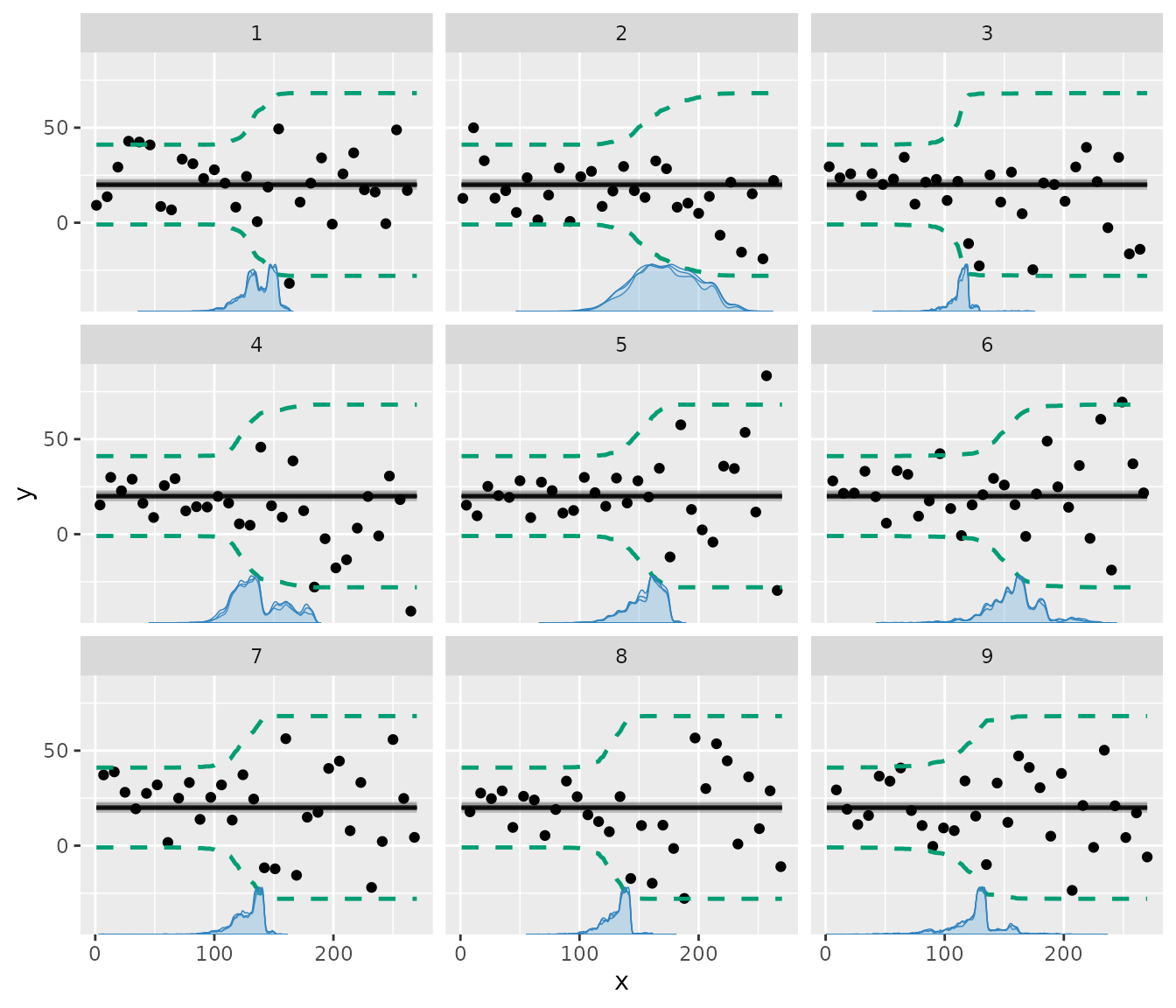

As usual, we can get the group-specific change points using coef(fit), or their deviations from cp_1 using ranef(fit):

coef(fit)

## # A tibble: 9 × 12
##   parameter group_col level  mean    sd lower upper  rhat ess_bulk ess_tail   sim match
##   <chr>     <chr>     <chr> <dbl> <dbl> <dbl> <dbl> <dbl>    <dbl>    <dbl> <dbl> <chr>
## 1 cp_1      id        1      137.  13.6 106.   156.  1.00     2383     3561  148. OK   
## 2 cp_1      id        2      173.  27.2 122.   222.  1.00      877     2080  167. OK   
## 3 cp_1      id        3      113.  10.2  90.7  128.  1.00     1107      813  119. OK   
## 4 cp_1      id        4      137.  21.0 103.   180.  1.00     1893     3376  124. OK   
## 5 cp_1      id        5      155.  15.0 121.   175.  1.00     1679     2596  149. OK   
## 6 cp_1      id        6      159.  23.1 109.   211.  1.00     1043     1320  165. OK   
## 7 cp_1      id        7      128.  13.4  97.2  143.  1.00     2461     2247  107. OK   
## 8 cp_1      id        8      131.  11.2 104.   143.  1.00     2262     3118  131. OK   
## 9 cp_1      id        9      125.  22.1  72.8  163.  1.00     1211     1223  122. OK

… and verify via posterior predictive checks:

pp_check(fit, facet_by = "id")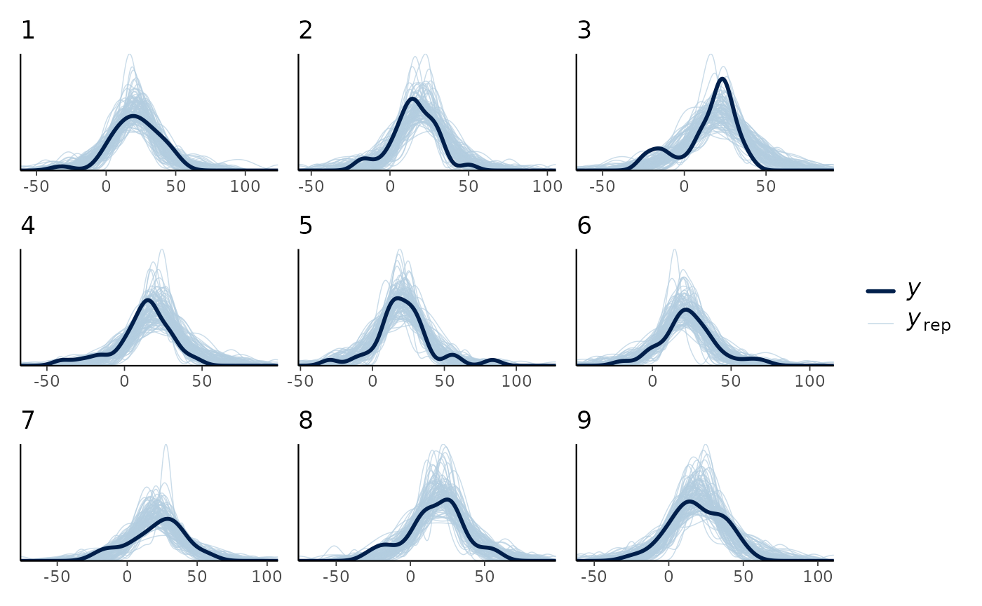

Generalizing to other distributional parameters (dpars)

sigma is just one instance of a distributional parameter in mcp. In general, every response family defines a set of supported dpars (distributional parameters). The default linear predictor in any segment formula models the location parameter mu (or probability/rate under the family’s link function). Other dpars can be regressed on predictors or given change points using wrapper functions named after the dpar.

Here is an overview of standard distributional parameters across response families:

mu: Conditional mean or location (e.g. mean for gaussian(), success probability for binomial(), event rate for poisson()). Modeled by default without any wrapper.
sigma: Residual standard deviation for gaussian() (modeled on the log-SD scale via sigma(...)).
shape: Overdispersion / shape parameter for negbinomial() (modeled on the log-shape scale via shape(...)).
ar() / ma(): Autoregressive and moving-average serial dependence terms for time-series models (read more here). Each lag is a dpar named ar1, ar2, ma1, etc. (see the definition above).

Inspecting and working with dpars

You can inspect the parameters of a model using mcp_pars(fit) and their priors using prior_summary(fit).

Many core mcp functions take a dpar argument to extract or visualize specific distributional parameters:

fitted(fit, dpar = "sigma") or fitted(fit, dpar = "shape"): Returns fitted values for the target dpar evaluated on the response scale.
plot_dpar(fit, dpar = "sigma") or plot_dpar(fit, dpar = "shape"): Plots the distributional parameter along the change-point variable, optionally with a central interval (interval = "fitted").

2026-10-26