
mcp aims to implement Generalized Linear Models in a way
that closely mimics that of brms::brm. You can set
the family and link functions using the family
argument.
First, let us specify a toy model with three segments:
model = list(
  y | trials(N) ~ 1,  # constant rate
  ~ 0 + year,  # joined changing rate
  ~ 1 + year  # disjoined changing rate
)
Simulate data
If you already have data, you can safely skip this section.
We run mcp with sample = FALSE to get what
we need to simulate data.
library(mcp)
future::plan(future::multisession, workers = 3)
set.seed(42)  # Make the script deterministic

df = data.frame(
  year = 1901:2020,  # evaluate for each of these
  N = sample(10:20, size = 120, replace = TRUE),  # number of trials
  y = 1
)

empty = mcp(model, data = df, family = binomial(), sample = FALSE)
Now we can simulate. First, let us see the model parameters.
empty$pars## List of 10
## $ x :"year"
## $ y :"y"
## $ cp :"cp_1" "cp_2"
## $ fixed :"Intercept_1" "year_2" "Intercept_3" "year_3"
## $ population:"cp_1" "cp_2" "Intercept_1" "year_2" "Intercept_3" "year_3"
## $ varying : NULL
## $ sigma :
## $ arma :
## $ trials :"N"
## $ weights : NULL- It takes two intercepts (
Intercept_*), for segments 1 and 3. - It takes two slopes (
year_*), for segment 2 and 3. - It takes two change points (
cp_*) - one between each segment.
empty$simulate is now a function that can predict data
given these parameters (signature:
empty$simulate(fit, newdata, ...)). If you are in a
reasonable R editor, type empty$simulate( and press TAB to
see the required arguments. I came up with some values below, including
change points at
and
.
Notice that because binomial() defaults to the link
function link = "logit", the intercept and slopes are on a
logit scale. Briefly,
this extends the narrow range of binomial rates (0-1) to an infinite
logit scale from minus infinity to plus infinity. This will be important
later when we set priors.
df$y = empty$simulate(
  empty, df,
  cp_1 = 1925, cp_2 = 1975,
  Intercept_1 = 2, Intercept_3 = -1,
  year_2 = -0.1, year_3 = 0.1)

head(df)
## year N y
## 1 1901 10 8
## 2 1902 14 13
## 3 1903 10 8
## 4 1904 18 15
## 5 1905 19 18
## 6 1906 13 13Visually:
plot(df$year, df$y)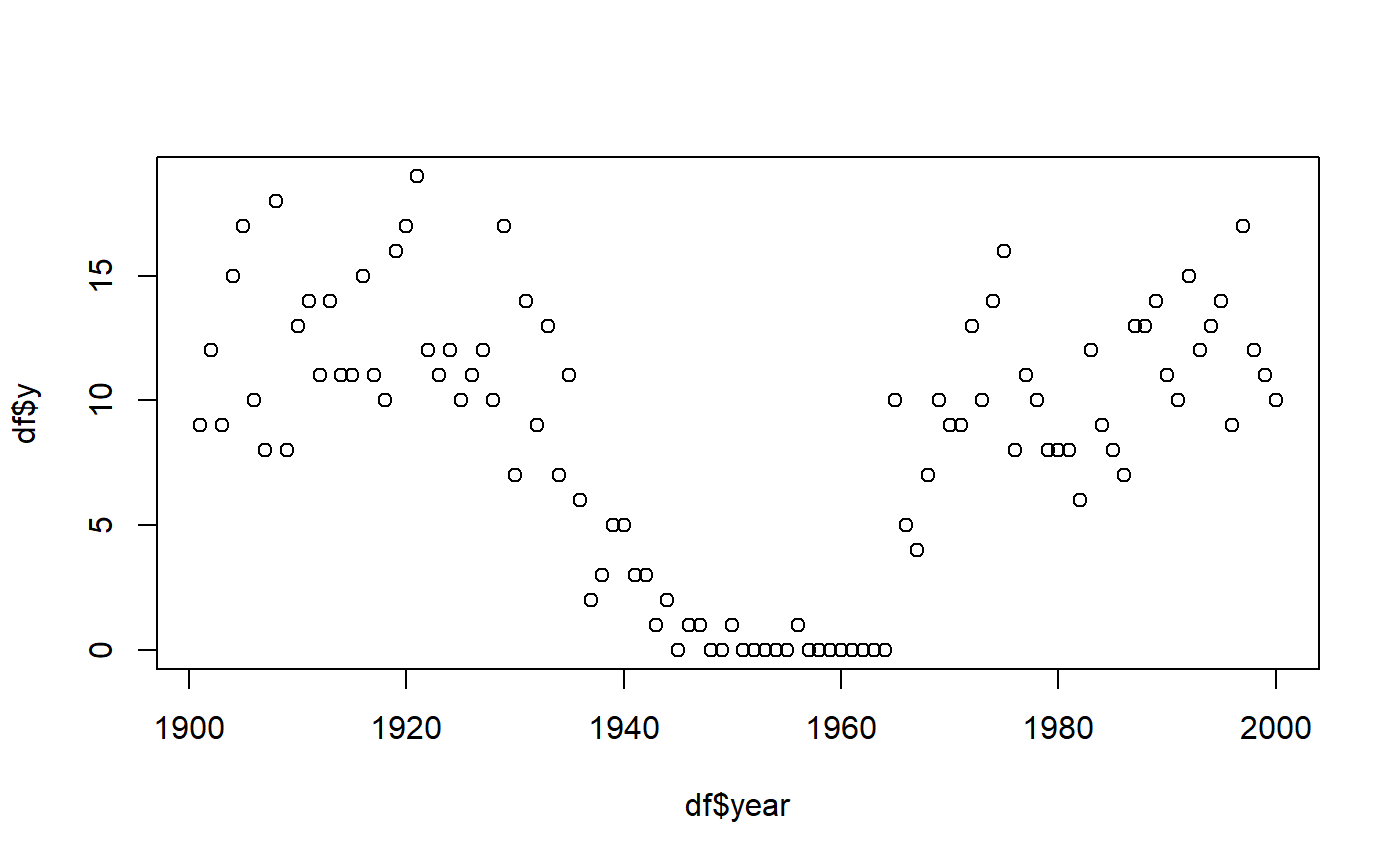
Check parameter recovery
The next sections go into more detail, but let us quickly see if we can recover the parameters used to simulate the data.
We can use summary to see that it recovered the
parameters to a pretty good precision. Again, recall that intercepts and
slopes are on a logit scale.
summary(fit)## Family: binomial(link = 'logit')
## Iterations: 9000 from 3 chains.
## Segments:
## 1: y | trials(N) ~ 1
## 2: y | trials(N) ~ 1 ~ 0 + year
## 3: y | trials(N) ~ 1 ~ 1 + year
##
## Population-level parameters:
## name match sim mean lower upper Rhat ess_bulk ess_tail
## cp_1 OK 1925.0 1921.756 1915.729 1927.613 1 316 765
## cp_2 OK 1975.0 1972.308 1960.533 1977.352 1 66 84
## Intercept_1 OK 2.0 2.179 1.818 2.582 1 526 1140
## year_2 OK -0.1 -0.093 -0.109 -0.079 1 386 699
## Intercept_3 OK -1.0 -1.497 -2.938 -0.712 1 70 80
## year_3 OK 0.1 0.112 0.093 0.130 1 380 1246
##
## Warning: 5 parameters show poor convergence (Rhat > 1.01 or ESS < 400).summary uses 95% central posterior intervals by default,
but you can change it using summary(fit, width = 0.80). If
you have varying effects, use
ranef(fit) to see them.
Plotting the fit confirms good fit to the data, and we see the discontinuities at the two change points:
plot(fit)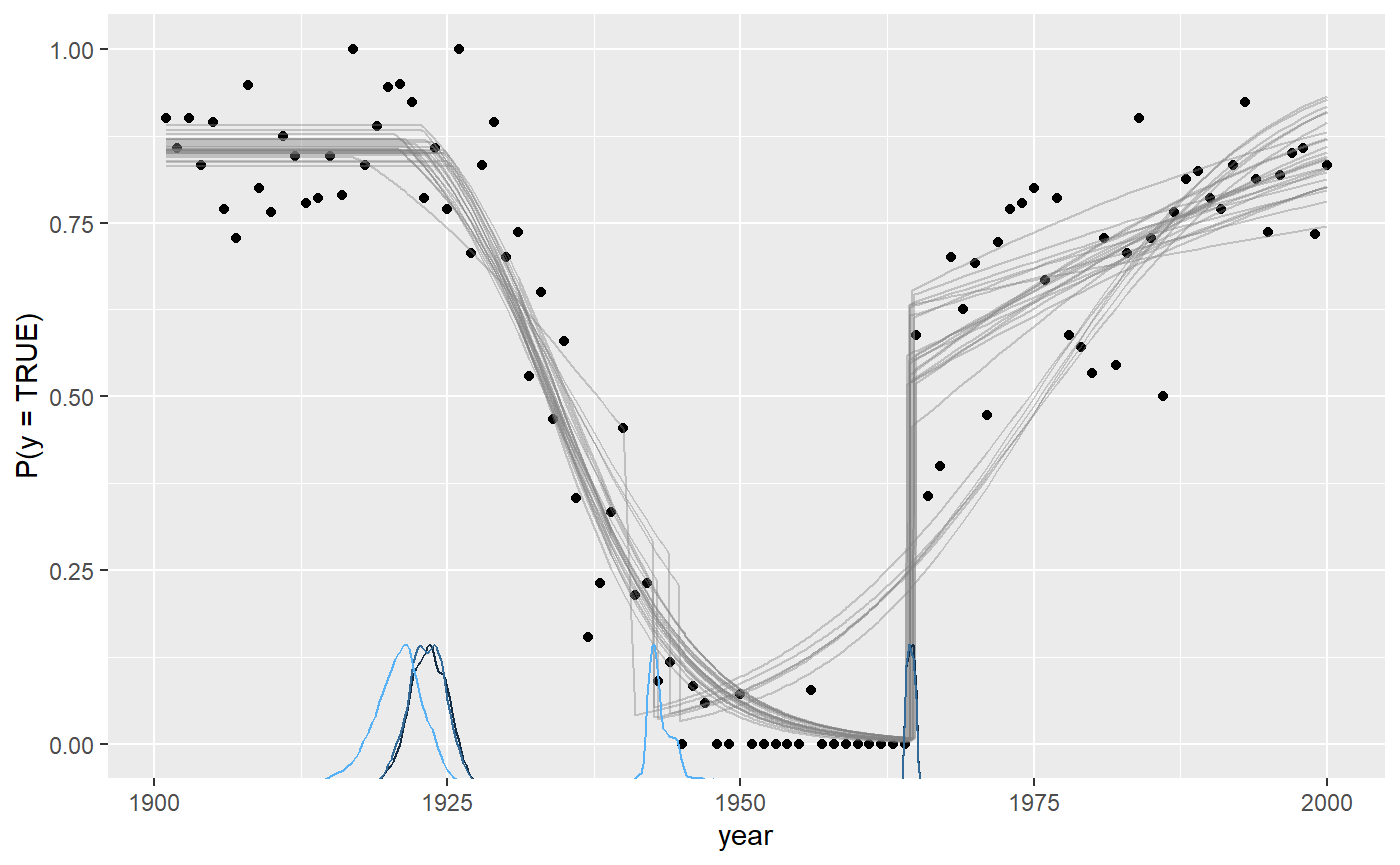
These lines are just fit$simulate applied to a random
draw of the posterior samples. In other words, they represent the joint
distribution of the parameters. You can change the number of draws
(lines) using plot(fit, lines = 50).
Notice for binomial models it defaults to plot the rate
(y / N) as a function of x. The reason why is obvious when
we plot on “raw” data by toggling rate:
plot(fit, rate = FALSE)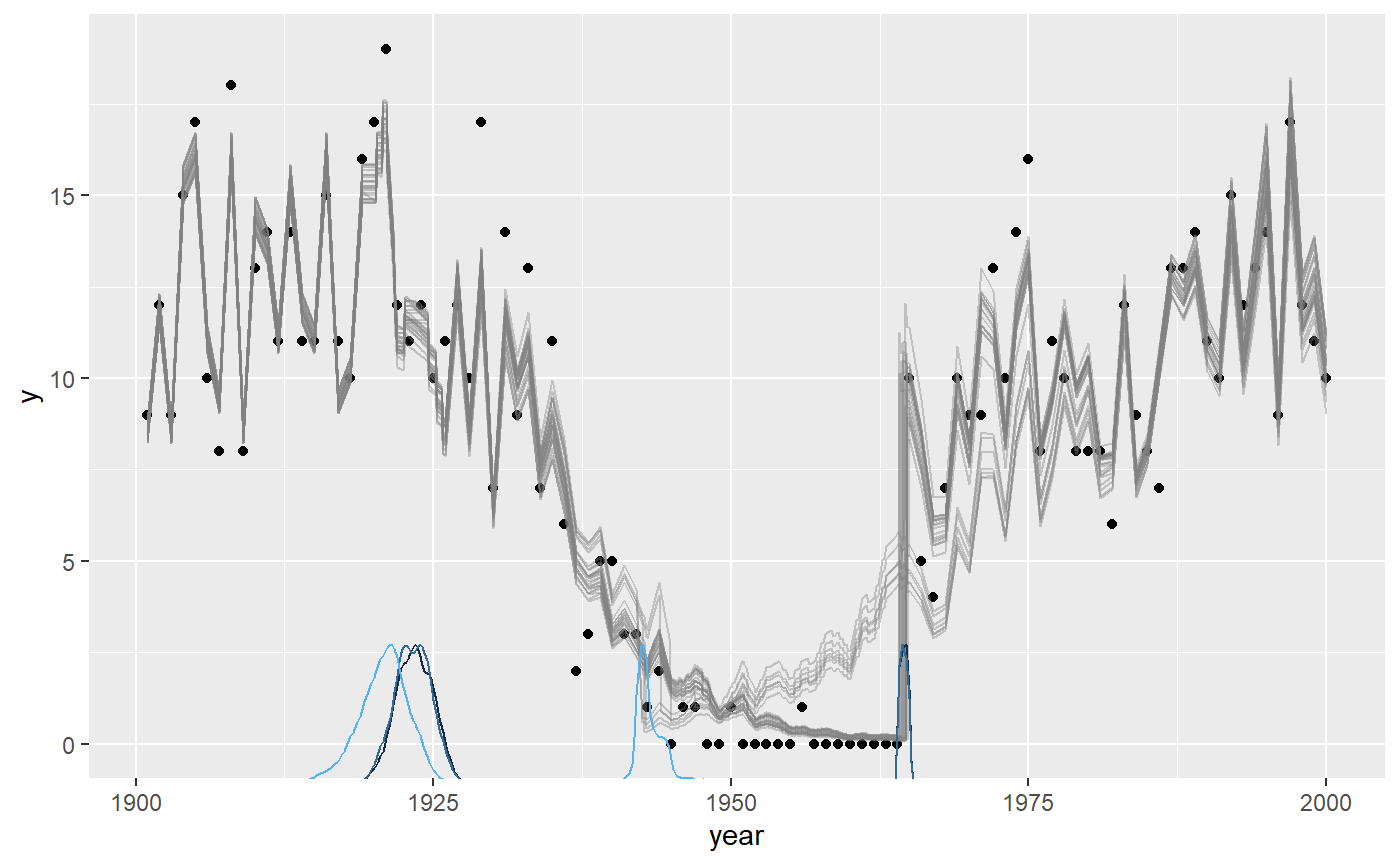
These lines are jagged because N varies from year to
year. Although there is close too 100% success rate in the years 1900 -
1920, the number of trials varies, as you can see in the raw data.
However, using rate = FALSE will be great when the number
of trials is constant for extended periods of time, as y is
more interpretable then.
Speaking of alternative visualizations, you can also plot this on the logit scale, where the linear trends are modeled:
plot_dpar(fit)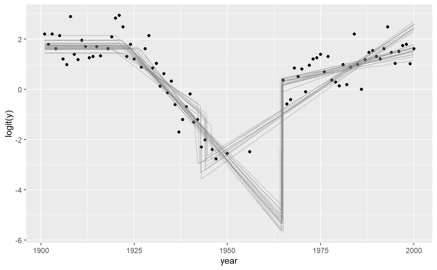
Of course, these plots work with varying effects as well.
Model diagnostics and sampling options
Already in the default plot as used above, it will be
obvious if there was poor convergence. A more direct assessment is to
look at the posterior distributions and trace plots:
plot_pars(fit)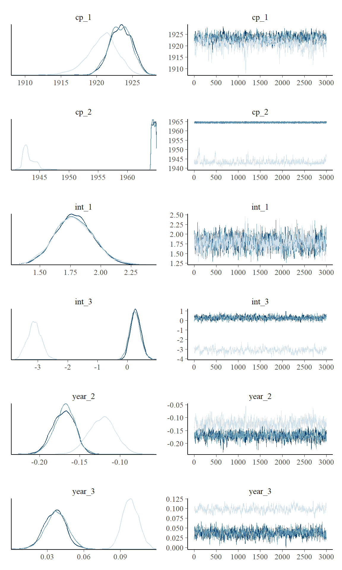
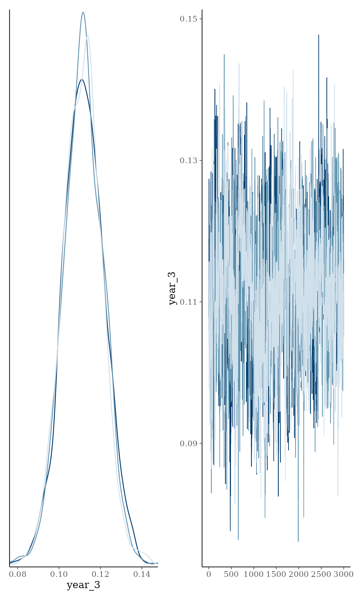
Convergence is perfect here as evidenced by the overlapping trace plots that look like fat caterpillars (Bayesians love fat caterpillars). Notice that the posterior distribution of change points can be quite non-normal and sometimes even bimodal. Therefore, one should be careful not to interpret the interval as if it was normal.
plot() and plot_pars() can do a lot more
than this, so check out their documentation.
Priors for binomial models
mcp uses priors to achieve a lot of it’s functionality.
See how to set priors, including
how to share parameters between segments and how to fix values. Here, I
post a few notes about the binomial-specific default priors.
The default priors in mcp are set so that they are
reasonably broad to cover most scenarios, though also specific enough to
sample effectively. They are not “default” as in “canonical”. Rather,
they are “default” as in “what happens if you do nothing else”. All
priors are stored in fit$prior (also
empty$prior). We did not specify prior above,
so it ran with default priors:
cbind(fit$prior)## [,1]
## cp_1 "dt(1901, 59.5, 1) T(1901, 2020)"
## cp_2 "dt(1901, 59.5, 1) T(cp_1, 2020)"
## Intercept_1 "dt(0, 1.5, 3)"
## year_2 "dt(0, 0.03781513, 3)"
## Intercept_3 "dt(0, 1.5, 3)"
## year_3 "dt(0, 0.03781513, 3)"The priors on change points are discussed extensively in the prior
vignette. With the default logit link, intercepts and categorical
contrasts use dt(0, 1.5, 3). Its central 95% interval is
approximately -4.8 to 4.8 logits, corresponding to probabilities from
0.008 to 0.992, while its heavy tails retain support for more extreme
values. The figure compares Student-t priors with scales 1 (red), 1.5
(black, the mcp default), and 2.5 (blue), together with
their correspondence to probabilities. The probit link currently uses
the same numerical default for simplicity.
Compared with the dt(0, 2.5, 3) intercept and flat
coefficient defaults in brms, these proper priors mildly
reduce extreme predictions in short segments while remaining broad and
heavy-tailed.
inverse_logit = function(x) exp(x) / (1 + exp(x))
scaled_t = function(x, scale) dt(x / scale, df = 3) / scale

# Start the plot
library(ggplot2)
ggplot(data.frame(logits = 0), aes(x = logits)) +

  # Plot Student-t priors. Set scale in "args"
  stat_function(fun=scaled_t, args = list(scale = 1), lwd=2, col="red") +
  stat_function(fun=scaled_t, args = list(scale = 1.5), lwd=2, col="black") +
  stat_function(fun=scaled_t, args = list(scale = 2.5), lwd=2, col="blue") +

  # Set the secondary axis
  scale_x_continuous(breaks = -7:7,limits = c(-7, 7), sec.axis = sec_axis(~ inverse_logit(.), name = "Probability", breaks = round(inverse_logit(seq(-7, 7, by = 2)), 3)))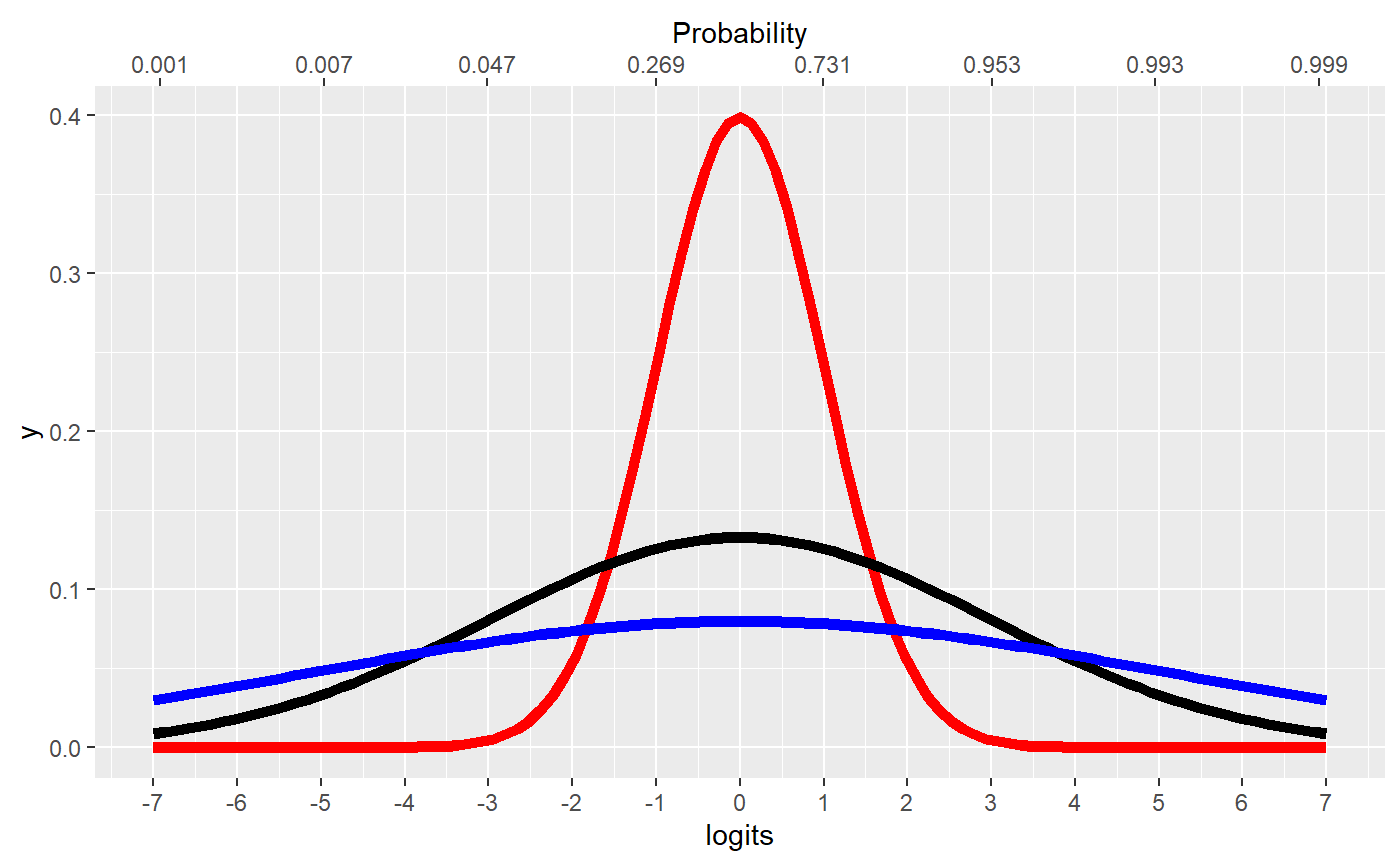
Please keep in mind that when these priors combine through the model, the joint probability may be quite different.
Numeric coefficient scales are divided by a representative change in
their model-matrix column: its range when it has two values, and two
standard deviations otherwise. Terms involving local par_x
additionally use the expected segment width,
(max(x) - min(x)) / n_segments(). The implied change across
a typical segment therefore has the same 1.5-logit scale, even when the
model contains several change points.
JAGS code
Here is the JAGS code for the model used in this article.
fit$jags_code## model {
## # mcp helper values
## cp_0 = CONST1_
## cp_3 = CONST2_
##
## # Priors for population-level effects
## cp_1 ~ dt(CONST1_, 1/(CONST3_)^2, CONST4_) T(CONST1_,CONST2_) # Within the observed change-point span
## cp_2 ~ dt(CONST1_, 1/(CONST3_)^2, CONST4_) T(cp_1,CONST2_) # Ordered after cp_1 within the observed change-point span
## Intercept_1 ~ dt(0, 1/(1.5)^2, 3) # Weakly regularizing link-scale intercept
## year_2 ~ dt(0, 1/(0.03781513)^2, 3) # Weakly regularizing link-scale coefficient scaled to a reference predictor change
## Intercept_3 ~ dt(0, 1/(1.5)^2, 3) # Weakly regularizing link-scale intercept
## year_3 ~ dt(0, 1/(0.03781513)^2, 3) # Weakly regularizing link-scale coefficient scaled to a reference predictor change
##
## # Model and likelihood
## for (i_ in 1:length(year)) {
## # par_x local to each segment
## x_local_1_[i_] = min(year[i_], cp_1)
## x_local_2_[i_] = min(year[i_], cp_2) - cp_1
## x_local_3_[i_] = min(year[i_], cp_3) - cp_2
##
## # Formula for mu
## link_mu_[i_] =
##
## # Segment 1: y | trials(N) ~ 1
## (year[i_] >= cp_0) * (year[i_] < cp_2) * inprod(rhs_matrix_[i_, c(1)], c(Intercept_1)) * 1 +
##
## # Segment 2: y | trials(N) ~ 1 ~ 0 + year
## (year[i_] >= cp_1) * (year[i_] < cp_2) * inprod(rhs_matrix_[i_, c(2)], c(year_2)) * x_local_2_[i_] +
##
## # Segment 3: y | trials(N) ~ 1 ~ 1 + year
## (year[i_] >= cp_2) * inprod(rhs_matrix_[i_, c(3)], c(Intercept_3)) * 1 +
## (year[i_] >= cp_2) * inprod(rhs_matrix_[i_, c(4)], c(year_3)) * x_local_3_[i_]
##
## # Likelihood and log-density for family = binomial()
## mu_[i_] = ilogit(link_mu_[i_])
## y[i_] ~ dbin(mu_[i_], N[i_])
## }
## }