This article introduces predict(), fitted(), residuals() for in-sample and out-of-sample data. I will also show how to get creative with mcp, including how to make predictions around future change points.
Preparation: an example model
We need an mcpfit to get started. We take the “demo” dataset:
library(mcp)
options(mc.cores = 3)  # Speed up sampling
set.seed(42)  # Make the script deterministic

ex = mcp_example("demo")
head(ex$data)
## # A tibble: 6 x 2
##    time response
##   <dbl>    <dbl>
## 1  68.4    32.8
## 2  87.3    -1.16
## 3  69.0    27.6
## 4  11.6    10.1
## 5  19.5    14.1
## 6  46.1    18.3
… and model it as three segments, i.e., two change points:
# Define the model
model = list(
  response ~ 1,  # plateau (int_1)
  ~ 0 + time,    # joined slope (time_2) at cp_1
  ~ 1 + time     # disjoined slope (int_3, time_3) at cp_2
)

# Fit it
fit = mcp(model, data = ex$data)
This is what the data and the inferred fit looks like with 95% credible interval and a 80% prediction interval:
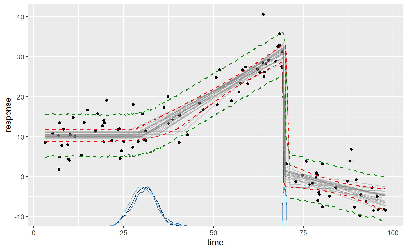
To review what we see here:
- The black dots is the data from
ex$data. - The gray lines are 25 samples from the posterior (control using
plot(fit, lines = 100)). - The dashed red lines are the 2.5% and 97.% quantiles of the fitted (expected) values.
- The green lines are the 10% and 90% quantiles of the predicted values.
- The blue curves on the x-axis are the posterior distributions of the change point locations (better viewed using
plot_pars(fit, pars = c("cp_1", "cp_2"))).
Behind the scenes, plot() merely calls predict() and fitted() to show these inferences.
Extracting fitted() values
To get the fitted values for each data point, simply do fitted(fit):
##       time    fitted     error      Q2.5     Q97.5
## 1 68.35820 30.352795 1.0524240 28.281702 32.375971
## 2 87.29038 -3.316264 0.7639949 -4.833468 -1.826587
## 3 69.01173 30.704731 1.0839745 28.566277 32.786091
## 4 11.59361 10.302963 0.7323588  8.826560 11.720457
## 5 19.50091 10.311477 0.7238347  8.878012 11.722323
## 6 46.12009 18.377166 1.0029739 16.038041 20.057603
In general, this output will include:
A column for each predictor column in the data. Here,
timeis the only predictor and you see the values in the same order as inex$data(which is copied tofit$data). But models with varying change points will additionally have a column for the varying data,binomial()models include the number of trials, etc.fitted: The fitted value which is the mean of the posterior for this predictor value (or set of predictor values). I.e., it is the Expected Value (EV).
error:: The standard error corresponding to
fitted, i.e.,diff(fitted + c(-1, 1) * error)is the 68% credible interval.Q[some number]: The quantiles of the fitted distribution. You can set the quantiles using
fitted(fit, probs = c(0.1, 0.5, 0.9)).
If you compare these values to the plot, you will see that they correspond. plot() merely calls fitted() behind the scenes.
Expected values for out-of-sample data
To predict out-of-sample data, you can simply use the newdata argument.
newdata = data.frame(time = c(ex$data$time[1], 25, -20, 200))
fitted(fit, newdata = newdata)
##       time    fitted      error       Q2.5     Q97.5
## 1  68.3582  30.35279  1.0524240  28.281702 32.375971
## 2  25.0000  10.34998  0.7175872   8.967093 11.770927
## 3 -20.0000  10.30119  0.7382389   8.825298 11.720457
## 4 200.0000 -28.14998 10.6442779 -49.429380 -7.991097
Note that:
- We get one row per value of
time. - The first value for
timeis in the dataset. The values correspond to the same row infitted(fit)because that’s merely a shortcut to dofitted(fit, newdata = fit$data). - The second value (
time = 20) is within the observed region, but not in the dataset. - The third value (
time = - 20) is outside the observed region, butmcpmerely extends the first segment backwards in time. Because it’s a plateau, we see approximately the same values as fortime = 20. - The fourth value (
time = 200) is way outside the observed region. Because it is the extrapolation of the slope in the third segment of which we’ve only observed the first tiny bit, the posterior distribution is very wide because even a small uncertainty in the slope results in very large differences further out.
Arguments
If you look at the documentation for predict(), fitted(), and residuals(), you’ll see that they are quite versatile, taking many different arguments. To mention a few, you can set which_y = "sigma" to get fitted values for sigma more on modeling sigma, prior = TRUE to predict using only the prior, varying = TRUE and arma = FALSE can be toggled to include/exclude AR(N) and varying effects.
Predictions
predict() is the posterior predictive and it takes exactly the same arguments as fitted(). This means that you can make predictions for in-sample and out-of-sample data as well. As with fitted(), plot() uses predict() under the hood to plot prediction intervals. You can see that the values correspond to dashed green lines in the plot (the 80% prediction interval):
##       time   predict    error       Q10       Q90
## 1 68.35820 30.275914 4.184053 24.972560 35.608088
## 2 87.29038 -3.339362 4.101321 -8.619435  1.880431
## 3 69.01173 30.764242 4.148573 25.449155 36.020085
## 4 11.59361 10.269686 4.077599  5.100657 15.494820
## 5 19.50091 10.195011 4.107429  4.956546 15.454846
## 6 46.12009 18.388889 4.124531 13.147433 23.702492
Note that predict() uses random sampling under the hood, so these values will differ slightly from call to call. You can make it replicable using set.seed() as above. In general, the more posterior samples, the less the call-to-call variance will be. Conversely, fewer samples means more call-to-call variation, e.g., if you do predict(fit, nsamples = 10)).
Residuals
residuals() is simply data$response - fitted(). It may be useful for model checking, but the typical needs are covered using posterior predictive checking (pp_check(fit)) and visual inspection of plot(fit, q_fit = TRUE, q_predict = TRUE).
Forecasting with future change points
Bayesian inference is the principled updating of prior knowledge using data. Where there is little or now data, the prior speaks louder. Sometimes, we can learn surprising stuff simply by inspecting the prior predictive, e.g., how the priors combine when “put through” the model. In mcp, most functions come with a prior = FALSE default, but you can simply do plot(fit, prior = TRUE), fitted(fit, prior = TRUE), or predict(fit, prior = TRUE).
Say you want to forecast at time = 125 and you know that a changepoint to the baseline level (an intercept change to int_1) will occur approximately after the same interval as between cp_1 and cp_2 (i.e., at cp_2 + (cp_2 - cp_1). Here is a way to “hack” mcp to do this. (NOTE: I plan on implementing this in a much more user-friendly way in a future release; see the discussion in this github issue and current status in this github issue).
Step 1: run the model for observed data
We already did that above, resulting in our fit. But we only do it to get the default priors that are suitable for inferring change point in this region, so you could’ve just run it without sampling:
fit = mcp(model, data = ex$data, sample = FALSE)
Step 2: add the unobserved segment(s) and fit
Now we extend the model with the future segment of which we have prior knowledge:
And finally, we extend the list of priors with the two new parameters (time_4 and cp_3). It may be helpful to review the article on priors in mcp.
prior_forecast = c(fit$prior, list(
  int_4 = "int_1",  # Return to this value
  cp_3 = "dnorm(cp_2 + (cp_2 - cp_1), 20) T(MAXX, )"  # In the future at the same interval
))
Now let’s fit it:
fit_forecast = mcp(model_forecast, data = ex$data, prior = prior_forecast)
Step 3: predict!
We can go right ahead and compute our 50% and 80% prediction intervals at time = 125:
predict(fit_forecast, newdata = data.frame(time = 125), probs = c(0.1, 0.25, 0.75, 0.9))
##   time  predict    error      Q10       Q25      Q75      Q90
## 1  125 3.946098 10.99492 -13.8512 -5.578755 11.79398 14.61287
To really understand what’s going on here, it may be helpful to visualize the model. For now, we will have to hack this a bit too, manually doing our plot:
# Get posterior and posterior predictive "predictions"
newdata = data.frame(time = 1:170)
fitted_forecast = fitted(fit_forecast, newdata = newdata, summary = FALSE, nsamples = 50)
predict_forecast = predict(fit_forecast, newdata = newdata, summary = FALSE)

# Plot it
library(ggplot2)
ggplot(predict_forecast, aes(x = time, y = predict)) +
  # Prediction intervals and line at x = 125
  stat_summary(fun.data = median_hilow, fun.args = list(conf.int = 0.8), geom = "ribbon", alpha = 0.2) +
  stat_summary(fun.data = median_hilow, fun.args = list(conf.int = 0.5), geom = "ribbon", alpha = 0.3) +
  geom_vline(xintercept = 125, lty = 2, lwd = 1) +

  # Lines for fitted draws
  geom_line(aes(y = fitted, group = .draw), data = fitted_forecast, alpha = 0.2) +

  # Observed data
  geom_point(aes(x = time, y = response), data = ex$data) +
  labs(title = "Predicting with future change points")
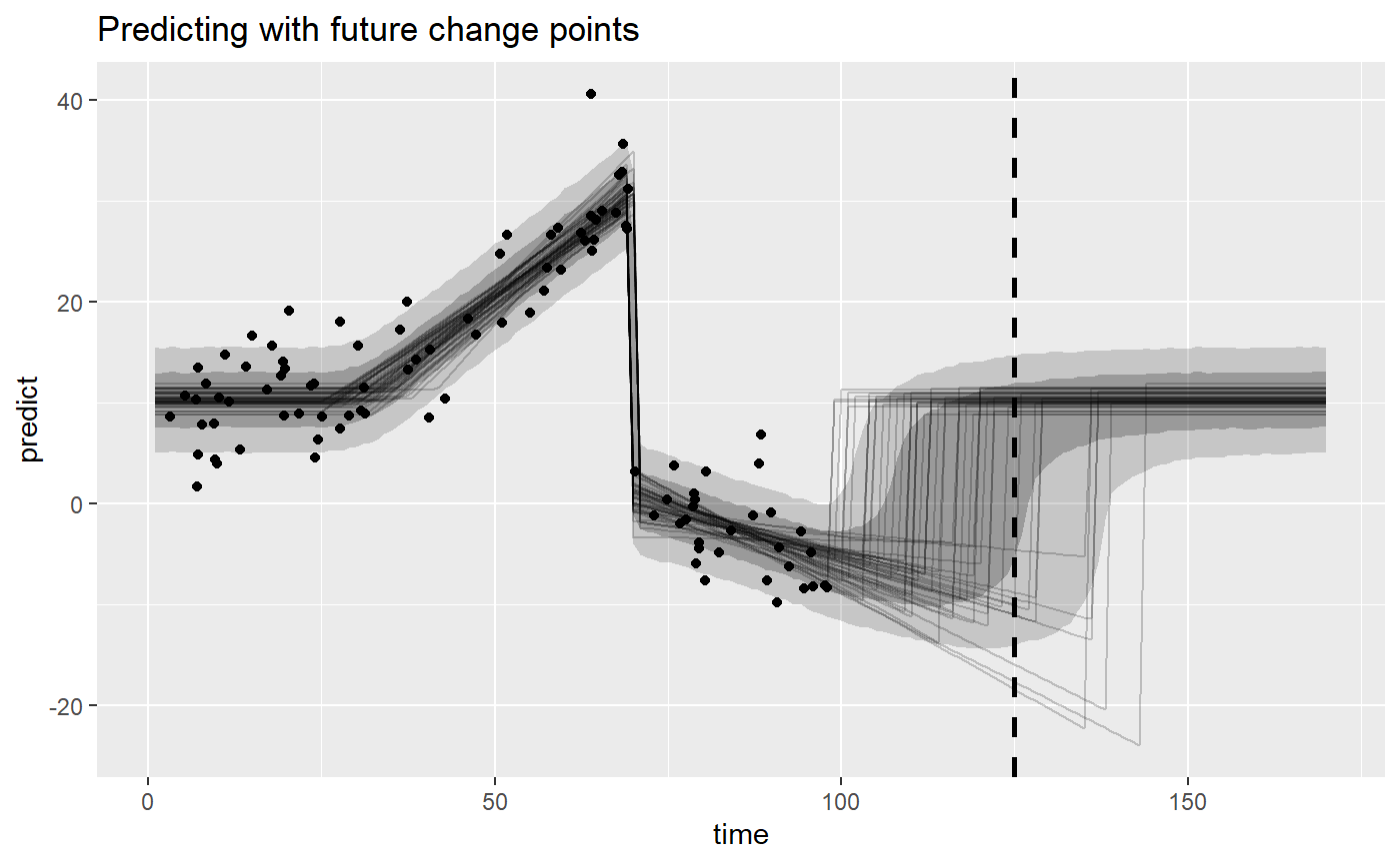
You can read the predicted values from above at x = 125 off this graph. We literally just predicted for all values between 1 and 170, and visualized it using a ribbon. This means that you can also predict further into the future, if you’d like.
You can extend this approach to an arbitrary number of future segments, even using the posterior from the “unobserved” segment 4 in the priors for parameters in future segments. In Bayesian inference, it really does not make much of a difference whether credence in some parameter values have been updated using data or not - it’s all credence.
Without doing this formal model of the future change point, one may have thought that the change point should occur around time = 110 since that’s the expected value of cp_2 + (cp_2 - cp_1). However, we truncated the prior for the future change point (cp_3) so that it occurs after the last data point (MAXX), i.e., at time > 100. This is knowledge that the third change point had not yet been observed at time = 100, and this pushes the distribution further into the future (actually around 118; see summary(fit_forecast)).