Model formulas in mcp

The model argument of mcp() is a list of formulas, one for each segment. A change point is estimated between each pair of consecutive segments. This page describes how segments connect, the formula syntax, and the underlying model. See mcp-priors for priors on the resulting parameters.

Details

Here is the demo model (see mcp_example("demo")):

model = list(
  response ~ 1,  # Plateau in the first segment (Intercept_1)
  ~ 0 + time,    # Joined slope (time_2) in segment 2 which starts at cp_1
  ~ 1 + time     # Disjoined slope (Intercept_3, time_3) at cp_2
)

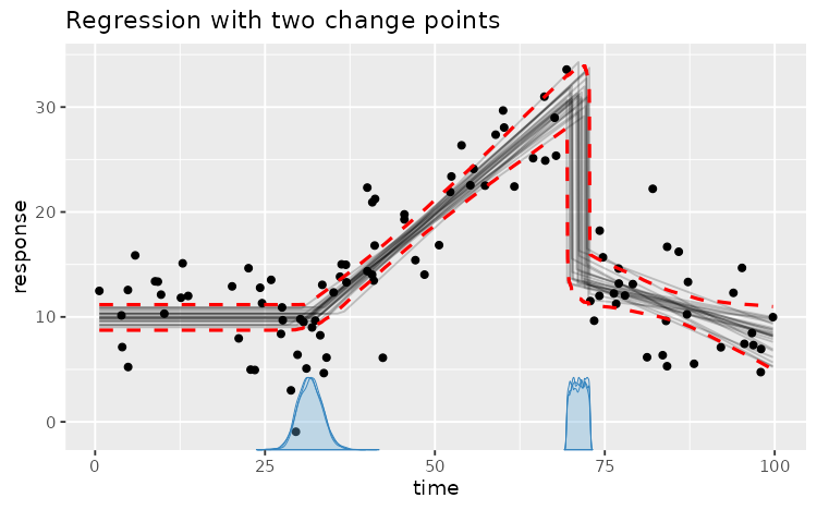
Fitted 3-segment mcp model with a plateau, joined slope, and disjoined slope

Segment 2 continues from where the plateau left off, while segment 3 starts afresh with a new intercept.

The modeling options and behavior are described below. They are described in a more applied and comprehensive way on the mcp website.

Three rules govern how segments connect (with x as the change-point variable, i.e., time above):

Only included terms get coefficients. A segment includes the terms in its formula, plus an intercept unless removed with 0 +. Each included term gets a new coefficient (x_2, stateB_2) or reuses an existing one if wrapped in same().
x-terms are measured from the change point. Only x, x:z, state:x, and I(x^2) start at zero at the segment's change point and stop growing at the next change point.
Joined or disjoined. Without an intercept (0 + ...), a segment is joined: it continues from where the earlier intercept and x-terms left off. With an intercept, it is disjoined and starts afresh.

sigma and shape are required by the likelihood, so they include an intercept in segment 1. They are joined in later segments that do not include them. ar() and ma() are not required, so a segment that does not include them has no AR/MA component. Each segment after the first starts at a change point, so it always includes a change-point intercept (cp_1, cp_2, ...). Use cp() to add terms to it, e.g., cp((1 | id)).

Formula syntax. The first segment has the format response ~ predictors. Later segments use the same response, so they are one-sided, ~ predictors, and each starts at a change point that can be modeled using cp(), e.g., ~ cp((1 | id)) + 0 + x. cp() is the change-point part of the formula and the rest is the predictor part.

1. Response (segment 1 only):

y ~ ...: Standard continuous, binary, or count response (Gaussian, Bernoulli, Poisson, negative binomial).
successes | trials(total) ~ ...: Binomial response (family = binomial()). Read more.
y | weights(w) ~ ...: Observation log-likelihood weights (multiplies each observation's log-likelihood contribution by w > 0; affects posterior inference and log_lik(), but not predictions).
y | trials(total) + weights(w) ~ ...: Combine response auxiliaries using +.

2. Change-point part (cp(), segments 2+):

~ x (i.e., cp() not included): Population-level change point (default). Same as ~ cp(1) + x.
~ cp((1 | id)) + x: Group-level change-point deviations around the population-level change point. Read more.

3. Predictor part (all segments): Read more

~ 1 + x: Disjoined slope with a new segment intercept.
~ 0 + x: Joined slope (no new intercept).
~ 1: Plateau (intercept only, no slope).
~ x:state + I(x^2) + exp(z): Extended terms, interactions, and R-side bases (scale(), poly(), splines::ns()). Bases are evaluated before sampling and reused for newdata. Except for I(x^k), transformations of x (e.g., I(x / 2)) use the original values of x, as in lm(), and do not join.
~ 1 + offset(log(exposure)): Offset with a fixed coefficient of 1. If one segment includes an offset, all segments must include one. The same applies within sigma(), etc., and within ar()/ma() in the segments that include them. Read more.
~ 1 + (1 | id): Group-level intercepts (or (1 + x || id) for independent slopes and intercepts). Read more.
~ sigma(1 + x): Distributional parameters on the link scale (e.g., log residual SD), with coefficients sigma_Intercept_2 and sigma_x_2. Without sigma() anywhere in the model, sigma_1 is the residual SD itself. Read more.
~ ar(1) + ma(1): Autoregressive and moving-average time-series residuals on the link scale (accepts regression formulas; include them in every segment where they apply). Set series = id and threshold once in any term; they apply to all segments. Read more.
~ 1 + same(x) or ~ 0 + same(z, as = 1): Reuse a coefficient from the preceding segment (default) or from segment as. Reused coefficients are estimated jointly from all segments where they are included, not fitted in one segment and copied to another. Read more.

The mcp model

An mcp model divides the change-point variable $x$ into $K$ segments separated by ordered change points $\tau_1 < \dots < \tau_{K-1}$. In each segment $k \in \{1, \dots, K\}$, the linear predictor $\eta_i$ measures $x$ from the change point $\tau_{k-1}$:

$$\eta_i = \alpha_k + \beta_{k,1} (x_i - \tau_{k-1}) \quad (\text{with } \tau_0 = 0)$$

where $\alpha_k$ is the value at the start of segment $k$:

$$\alpha_k = \begin{cases} \beta_{k,0}, & \text{disjoined } (\sim \texttt{1 + x}, \text{ or } k = 1) \\ \alpha_{k-1} + \beta_{k-1,1} (\tau_{k-1} - \tau_{k-2}), & \text{joined } (\sim \texttt{0 + x}) \end{cases}$$

That is, a disjoined segment starts at its own intercept $\beta_{k,0}$, while a joined segment continues from where segment $k-1$ left off.

Here, $\beta_{k,1}$ is the slope on $x$ in segment $k$. Intercepts and slopes are absolute values (not changes relative to preceding segments). Other variables (e.g., + z + state) add $\sum_j \gamma_{k,j} z_{j,i}$ in the segments where they are included. They use their original values and are not part of $\alpha_k$, which is why they can make a joined segment start with a jump.

The inverse-linked parameter is $\mu_i = g^{-1}(\eta_i)$ via link function $g(\mu_i) = \eta_i$, representing the expected response for most families (or the success probability for binomial models, where the expected count is $n_i \mu_i$). Distributional parameters (sigma(), shape(), etc.) and autoregressive terms (ar(), ma()) follow this exact same segmented structure on their respective link scales. Since each of them has its own segmented linear predictor, mcp calls them all distributional parameters (dpar): mu, sigma, shape, and each AR/MA lag (ar1, ar2, ma1, ...), e.g., fitted(fit, dpar = "ar1") or fixef(fit, dpar = "sigma"). See more details on the mcp website.

Time-series residuals (link-scale observation-driven GARMA)

Autoregressive (ar(p)) and moving-average (ma(q)) terms define a finite conditional recurrence on the link scale (generalized autoregressive moving-average, GARMA). They support Gaussian (identity), binomial (logit), Bernoulli (logit), Poisson (log), and negative-binomial (log) families. If $\eta^{\text{reg}}_t$ is the ordinary linear predictor from the segment formulas and $\eta_t$ is the linear predictor including serial dependence, the recurrence decomposes into components:

$$\begin{aligned} \text{AR}_t &= \sum_{j=1}^{p} \phi_{j,t} \left[g(y^*_{t-j}) - \eta^{\text{reg}}_{t-j}\right] \\ \text{MA}_t &= \sum_{k=1}^{q} \theta_{k,t} \left[g(y^*_{t-k}) - \eta_{t-k}\right] \\ \eta_t &= \eta^{\text{reg}}_t + \text{AR}_t + \text{MA}_t \end{aligned}$$

where $\phi_{j,t}$ is the lag-$j$ autoregressive (AR) coefficient at time $t$, $\theta_{k,t}$ is the lag-$k$ moving-average (MA) coefficient at time $t$, $g(\cdot)$ is the link function, and $y^*_t$ is the observation, constrained by a threshold constant $c$ (argument threshold = 0.1 in ar() / ma()) to keep residuals finite on the link scale, e.g., $y^*_t = \max(y_t, c)$ for zero counts in Poisson models. Read more.

Implications:

For an $N$-order component, the last $N$ values before the segment's change point are input to the first $\eta_t$ in the segment.
AR and MA components apply only in segments where they are included.
AR coefficients are not jointly constrained to stationarity; nor MA coefficients to invertibility.
See the arma article for more details.

Details

The mcp model

Time-series residuals (link-scale observation-driven GARMA)

See also